Good Math Problems

Folium of Descartes

Today, actually just an hour or so ago, another math teacher asked me if I knew a way to parametrize the following:

$x^3+y^3=3xy$

It is also known as the Folium of Descartes and looks like:

Her purposes was just trying to find a quick and easy way to graph it on the calculator. It was just a small, unimportant question. She didn’t need to know the answer, if it wasn’t easily doable. But to me, I needed to know! How do we find the parametric equations which define this? I just don’t know. The answer I found online is:

$x(t)=\frac{3t}{1+t^3}$ and $y(t)=\frac{3t^2}{1+t^3}$

And it’s pretty easily verifiable when you work backwards with the parametrization.

Is there something I’m missing? Is there a method to working from implicitly defined 2D functions to parametrizations for them?

sin(1/x)

In my most recent calculus classes, I wanted to show my kids their first “not nice” functions. After being introduced to how to find limits graphically (fancy way of saying: looking at the graph of a function) and numerically (fancy way of saying: using the graphing calculator’s TABLE function to guesstimate limits), I wanted to have them think about what they learned.

I had time to show one class that these methods aren’t foolproof — that the calculator can lie to you, and make you think a limit is 3 when it is in fact 3.004, or that it can’t graph things when numbers get too large or too small. So they have to be careful. And that we will be learning algebraic methods to do limits. But for now, they need to use their brains and wits.

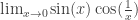
So I divided them into groups of 2 and 3 and had them use whatever methods they wanted to find:

$\lim_{x \to 0} \sin(\frac{1}{x})$

I made them each draw a sketch of the function, write down an appropriate table of values, make observations about the function, and then decide on an answer. (In one class, I had each group turn in their findings, and then I photocopied them and distributed them and had the class talk collectively about the results the next day. In the other class, we didn’t have time for this, and we just met up together as a group to talk.)

FYI, the graph is here.

It was great. Students were debating whether the craziness was a function of the calculator lying or if that actually was what the function looked like. They wondered if the limit was 0 or if it was “does not exist.” They noticed that the function starts to oscillate more and more rapidly as $x$ approaches 0. They noticed that it bounced between -1 and 1. It’s not an easy question to solve with this information.

When we came back as a group, we talked about their observations and conclusions, and documented them on the board — so everyone had the same notes. Then I said: “so… one of you said that the function is crossing the $x$ axis more and more as $x$ is getting closer and closer to 0. Can we be more exact? Where does the function cross the $x$ axis?”

Of course my students didn’t know exactly what to do. We got to the point where we knew we had to solve:

$\sin(\frac{1}{x})=0$

But then they were stuck. So I guided them through it.

I asked: “When is $\sin(\square)=0$

We generated: $\square=...,-4\pi,-3\pi,-2\pi,-1\pi,0,1\pi,2\pi,3\pi,4\pi,...$

We then said: $\frac{1}{x}=...,-4\pi,-3\pi,-2\pi,-1\pi,0,1\pi,2\pi,3\pi,4\pi,...$

We went through solving one of the equations for $x$ and saw that we needed the reciprocals…

We concluded: $x=...,\frac{-1}{4\pi},\frac{-1}{3\pi},\frac{-1}{2\pi},\frac{-1}{1\pi},\frac{1}{\pi},\frac{1}{2\pi},\frac{1}{3\pi},\frac{1}{4\pi},...$

I then asked: So what? Why did we do this? Don’t lose the forest for the trees…

Finally, we converted those numbers to decimal approximations

$x \approx \pm 0.318,\pm 0.159,\pm 0.106, \pm 0.080, \pm 0.064, \pm 0.053, \pm 0.045, \pm 0.040, ...$

and saw that the zeros were getting more and more frequent as we approached 0. No matter how close we came to zero, we were still going to be bobbing up and down on the function. And crucially, we’ll be bobbing up and down between $-1$ to $1$ .

We then talked about what a limit means again… what the $y$ value of a function is approaching as the $x$ value gets closer and closer to a number. Using that informal definition, I asked them if the $y$ value of the function was approaching some number as $x$ was approaching 0.

At this point, most of my kids had that “a hah” moment.

I am definitely doing this again next year, but perhaps more formalized. I might generate a list of good conceptual questions to walk them through this more systematically. One such question: “How many zeros are there in the interval (.5,1)? How about (.1,1)? How about (.01,1)? How about (.001,.1)? How about (0.0001,1)? And finally, how about (0,1)?” Another such question: “How do we know the function will bounce between $-1$ and $1$ ?”

Also, maybe next year, I’ll couple it with an analysis of the function:

$\lim_{x \to 0} \sin(x)\cos(\frac{1}{x})$

The function behaves similarly (crosses the $x$ axis more and more rapidly as $x$ approaches 0), but the limit in this case is 0. You can see it in the graph easiest.

So if anyone out there is looking for something to spice limits up, you might want to really go in depth into these functions. They are often used as exemplars, but rarely investigated.

A Great Calculus Problem… that is Powerfully Related to Geometry

I’m sitting in a building at Exeter, digesting lunch and waiting for the next session to begin. I’m at what has so far been a really valuable math teacher conference. What impresses me most, besides the amazing and neverending supply of food that they offer, is the population of teachers that come. Many of the teachers I’m talking with have 20+ years of experience in the classroom.

Over the next few days I’m going to use this blog to talk about some of the tidbits of interesting problems I’ve been presented with, to good resources or programs that I was introduced to, to neat ways to present topics in class, to ideas that I’ve been inspired to think about.

I’m going to start with a nice calculus problem — probably good for a AP Calculus BC class, but there is definitely a way I could show this problem to my non-AP class.

Here’s the problem. You’re in a museum and you’re looking at a painting which is hung above eye level. (There is a specific painting which is hung high in the entrance room at the Brooklyn Museum that I think of with this problem.) You are standing some distance away from it. The question is: what is the largest angle ( $\alpha$ ) that you can get as you walk forwards and backwards? (See diagram below for setup.)

So to be clear, as you move the eyeball forward and backwards along the dashed blue line, what’s the largest angle you can create? Of course if you walk right up to the painting, or far away, the angle is going to decrease to 0. If you can’t see that, look at the diagrams below.

So of course there has to be some perfect distance that will give you the maximal angle. You see where this is going…

Find that maximum angle! (Use the variables in the diagram below.)

Of course this doesn’t have to be a painting. It could be, as the speaker pointed out, an overhead view of a hockey rink, with the painting being the goal, and the eyeball being the player with a puck. Where does the hockey player have the maximum angle to shoot and make it into the goal?

I want you to have the fun of solving it, but the solution I came up with was:

$\alpha=\tan^{-1}(\frac{P}{2\sqrt{Y(P+Y)}})$

(I can help you with that if you want. Just throw your questions or cry for help in the comments.)

However, there is something pretty amazing about this problem, something that is powerfully seen with geometry software like geogebra or geometer’s sketchpad. Check out the sheet I made and see what happens as I bring the person close to the picture and look for the optimal angle? When you look at this, try to see if there is a geometry connection to our solution for the largest angle…

Vodpod videos no longer available.

more about “Geogebra_Picture_Problem“, posted with vodpod

Do you see the geometry connection? The optimal angle exists when the circle created by the top of the picture, the bottom of the picture, and the eyeball is tangent to the line of sight. Now my charge to you — which would be my charge to my students — is to (a) explain in words why this is true and (b) use geometry to calculate this optimal angle. You know, this work is an exercise for the reader. I mean, I’m not going to do everything for you. Sheesh.

Composition of Functions and their Inverses

In Algebra II, we have been talking about inverses, and compositions. We finally got to the point where we are asking:

what is $f^{-1}(f(x))$ and what is $f(f^{-1}(x))$ ?

Last year, to illustrate that both equaled $x$ , I showed them a bunch of examples, and I pretty much said… by the property of it working out for a bunch of different examples… that it was true. However, that sort of hand-waving explanation didn’t sit well with me. Not that there are times when handwaving isn’t appropriate, but this was something that they should get. If they truly understand inverse functions, they really should understand why both compositions above should equal $x$ .

So today in class, we started reviewed what we’ve covered about inverses… I told them it’s a “reversal”… you’re swapping every point of a function $(x,y)$ with $(y,x)$ . That reversal graphically looks like a reflection over the line $y=x$ . Of course, that makes sense, because we’re replacing every $y$ with an $x$ — and that’s the equation that does that. My kids get all this. Which is great. They even get, to some degree, that the domains and ranges of functions and their inverses get swapped because of this.

But then when I say:

“ $f(x)$ means you plug in $x$ and you get out $y$ … but then when you plug that new $y$ into your $f^{-1}(y)$ you’ll be getting $x$ out again”

their eyes glaze over and I sense fear.

So I came up with this really great way to illustrate exactly what inverses are and how the work… on the ground. I put up the following slide and we talked about what actually we were doing when we inputted an $x$ value into both the function and the inverse:

We came up with this:

We then talked about how we noticed that the two sides were “opposites.” Add 1, subtract 1. Multiply by 2, divide by 2. Cube, cube root. And, importantly, that they were in the opposite order.

Then we calculated $f^{-1}(f(3))$ :

Starting with the inner function: $f(3)$

(1) cube: 27
(2) multiply by 2: 54
(3) add 1: 55

Then we plugged that into the outer function: $f^{-1}(55)$

(1) subtract 1: 54
(2) divide by 2: 27
(3) cube root: 3

This way, the students could actually see how a composition of a function and its inverse actually gives you the original input back. They could see how each step in the function was undone by the inverse function.

I don’t know… maybe this is common to how y’all teach it. But it was such a revelation for me! I loved teaching it this way because the concept became concrete.[1]

[1] I remember reading some blog some months ago that was talking about solving equations, and how each step in an attempt to get $x$ alone was like unwrapping a present. I like that analogy, even though the particular post and blog eludes me. But in those terms, this is like wrapping a present, and then unwrapping it!

Take what you don’t know…

In Calculus, I sound like a broken record. Each time we learn something new, I say “take what you don’t know and turn it into what you do know.” I say that at least three times a week. I said it last week when doing integrals like:

$\int \frac{1}{4x^2+1} dx$

We don’t know how to deal with that, but we do know how to deal with

$\int \frac{1}{x^2+1}dx$

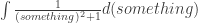
So let’s try to turn what we don’t know how to do into something we do know how to do. For those who haven’t taken calculus for a while, the integral above is $\tan^{-1}(x)+C$ . So to do the original problem, we want to somehow get the original integral to look like $\int \frac{1}{(something)^2+1}d(something)$ — the integral of 1 over something squared plus 1. So we rewrite the integral as $\int \frac{1}{(2x)^2+1}dx$ . That’s much closer to what we want to get — it looks more like something we know how to deal with. Next we use $u$ -substitution to finish this beast off ( $u=2x$ ) to get $\frac{1}{2} \int \frac{1}{u^2+1}du$ . Now we have something we know how to deal with, from something we didn’t.

Again today, I showed my students how to solve $\int_0^1 \sqrt{1-x^2}dx$ , and told them to solve: $\int_0^1 5-3\sqrt{1-x^2}dx$ . At first sight, they recoiled, but again, we used the mantra of “take what you don’t know and turn it into what you do know” to solve it. If it looks scary, fine, have a moment of panic, but then ask yourself “what does this look like” and “can I turn it into that with some simple manipulation”?

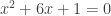
I was thinking today how this actually could be my refrain in Algebra II also. Example: I could frame quadratics in that way. Students know — or quickly learn — how to solve equations like $(x+1)^2=5$ (hopefully). But what about something like $x^2+6x+1=0$ ? It’s not nearly as easy. But then we can talk about if there is a way to that what we don’t know (that equation) and turn it into something we do know how to solve ( $(x+3)^2=8$ ). It’s not that I don’t do this already, but I am not always explicit about it. It is not my mantra.

But it should be. It’s how we solve math problems. We have something we don’t initially know how to do. And we have to figure out if we can simplify/rewrite/re-envision it to bring it to a place where we know how to do it.It seems stupid and simple and obvious, so much so, that I don’t say all the time. But if I started saying that as my refrain, if students really saw that math is simply this simple process, it might stop seeming like a huge bag of tricks that never fall together. They might see it as the art that it is — where there is creativity in deciding how to get from point A (hard problem) to point B (simple problem they know how to do). And all the specifics that we do in class are giving them the tools which they can use to chisel out a path from A to B. It might finally be us always trying to work out the puzzle: what does this look like that we know how to do, and can we get it to that place?

In other words, we’re now talking processes instead of methods. We’re talking problem solving instead of rote memorization. And whenever a student is stumped on a problem, you can stimulate his/her thought process by saying “we’ve always taken what we don’t know how to do and turned it into something we do know how to do… what similar things does this beast remind you of?”

So yeah, it’s not a huge revelation or anything. But I’m thinking that it might be a really amazing experiment to frame my Algebra II and Calculus classes with this mantra next year. Heck, maybe even in the next few weeks when I’m teaching exponential and logarithmic functions! I mean, yeah $\log(2x+1)+\log(x-1)=2$ may look ugly. But is there a way to turn it into something we do know how to do? Namely something of the form $\log(something)=2$ ? Obvi.

Moving Day!

I found a new apartment that I’m in love with, and I’m moving at the beginning of May. I called two moving companies which had been recommended to me to get price estimates.

Both will send 3 people.

Company A charges $100/hr for their services. However, they have a 2.5 hour minimum charge. They also charge $100 for 1 hour of travel time (30 minutes to the apartment and 30 minutes from the apartment). There is an additional fee of $50 for packing charges for my futon, mattress, and TV. Lastly, they charge by the quarter hour. So if they worked 151 minutes, they’d charge me for 2.75 hours.

Company B charges $130/hr for their services. They have a 2 hour minimum charge. They also charge a travel fee, but it is only $65 in total. Lastly, they too charge by the quarter hour. So if they worked 121 minutes, they’d charge me for 2.25 hours.

The question I was left with is: which is the better company for me to hire?

The only variable is the amount of time the movers spend moving.

The x-axis is the hours spent moving, the y-axis is the amount of money my bank account will be missing. Company A is in blue, Company B is in red.

What’s awesome is that we just taught functions and function transformations in my Algebra II class. And one of the functions we worked with a lot was the floor (step) function. We’ve also talked about piecewise functions. If I were teaching an accelerated class, I would literally give them the information and ask them to (a) first produce the graph, and then (b) from the graph, come up with a function that gives them the graph.

They’re going to have to recognize they’ll need a piecewise equation, and then also have to figure out how to make the function transformations on the step function to get the second half of the piecewise equation.

I kind of love this problem.

A fun double integral

On my multivariable calculus class’s current problem set, I put a number of really challenging problems. One of them — from both the Exeter Math 5 course (here) and also in Anton — has students evaluate the following double integral, and then has students change the order of integration and then evaluate the double integral.

$\int_0^1 \int_0^1 \frac{x-y}{(x+y)^3}dydx$

Students expect the answers to be the same, but it turns out they are not. (Do you see why?)

Anyway, I have to say that I’m not a master integrator; it usually takes me a little longer than desired to figure out the best method to integrating. But I enjoyed the roads I took, so I thought I’d share the integral with you if you wanted a challenge.

And for those of you who know calculus, but forgot or never learned multivariable calculus, the problem reduces to you solving the following single integral: $\int_0^1 \frac{a-y}{(a+y)^3}dy$ , where $a$ is just a constant.