I was in the middle of writing how I made the transition from Anti-Derivatives to Integrals, and then I got swept up with school things. So a month and a half later, at the start of my summer vacay (!), I’m going to write up the very last post in this installment, where I make The Final Turn.

As a recap: I taught anti-derivatives as “the backwards question” of derivatives, but didn’t give them any meaning other than a mathematical puzzle. And my first post (Part I) starts when I tell kids we’re going to put anti-derivatives aside for a while and we’re going to think about a road trip. In this, students recognize that velocity graphs can tell you about displacement, and we are forced to contend with left handed and right handed riemann sums. The conclusion is that “the displacement of an object can be calculated by estimating the area under a velocity graph.” Importantly, for kids, this has nothing to do with anti-derivatives. In my second post (Part II), students explore this idea in more detail. They are given a bunch of step functions for velocity and they come to recognize the difference between distance and displacement, and also why we need to specify a starting position to know an ending position. They also see the need for negative signed area to represent moving backwards. Again, this has nothing to do with anti-derivatives.

This is where our story begins. The final part of this tale, where we connect signed areas (which students are comfortable with) to anti-derivatives in such a way that the connection makes sense and is actually kinda obvious. That was my goal, anyway.

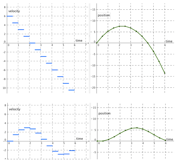
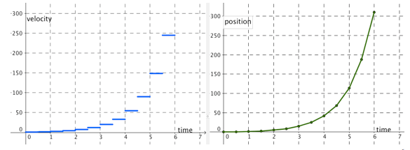
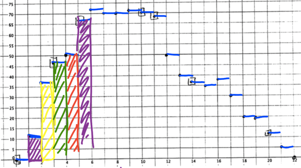
At the end of the same packet students were working on in Part II, I gave the following velocity and position graphs. Like my students, you can probably see that the velocity graphs are approximations of “nice” curves (e.g. quadratic, square root, linear, sine, exponential, cubic).

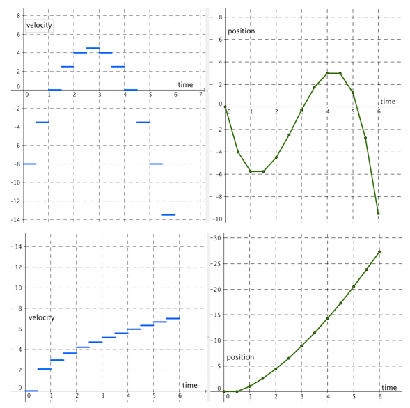
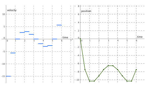
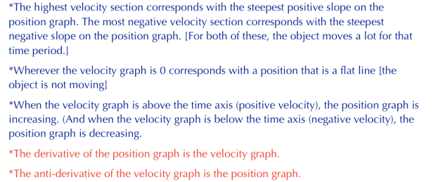
After being asked to identify some specific things on each graph (find what happens to the corresponding position piece when the velocity was greatest… find what happens to the corresponding position piece when the velocity was zero… etc.), I asked students to write six different things they noticed/observed. Kids came up with great observations! Here are some of them taken from their nightly work (note: “palley” is our class terminology for peak or valley):

• Zero on the velocity graph yields a slope of 0 on the position graph (the object didn’t move for that time period)
• Most positive value on the velocity graph yields the largest positive slope on the position graph
• Most positive value on the velocity graph corresponded with the largest change in position (from low to high) on the position graph
• The position graph usually has one more palley than the velocity graph (when we’re dealing with polynomial velocity graphs)
• When the velocity graph is negative, the position graph is decreasing
• When the velocity graph is positive, the position graph is increasing
• For the 4th graph, the velocity graph looks like a sine graph and the position graph looks like a cosine graph
• Many of the relationships between graphs look similar to derivatives we’ve been studying
• At the point of highest velocity, the position graph usually has a palley
• The area under the velocity graph gives the height of the position graph
• Velocity graph is the derivative of the position graph

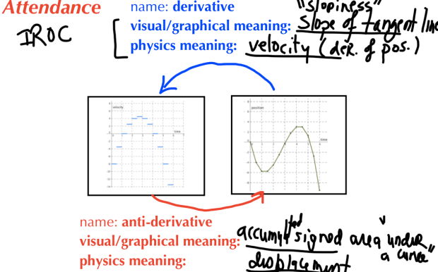
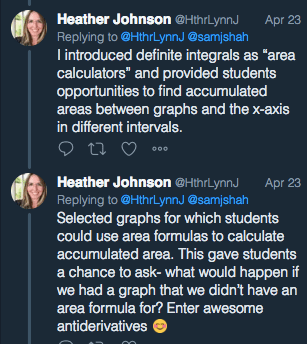
Ooooh! I just found the smartboard page where we codified these in one class:

To debrief this, I had kids call out their observations and we talked about them/refined them using the graphs I was projecting at the front of the room. The most important thing I remember doing was making sure we started with “simple” observations and only then had the class move to more “complex” observations. That way kids who only noticed basic things would have a chance to voice their thinking.

From this we finally got to the conclusion we were looking for: the velocity graph is the derivative of the position graph. I had to nudge kids to make the counter-observation they get for free: the position graph is the anti-derivative of the velocity graph.

We saw all the things we had previously learned when studying the shape of a graph come out (e.g. when the derivative is negative, the original function is decreasing; when the derivative was zero, the original function often had a “palley”). Everything fit together!

We then carefully looked at small pieces of one of the graphs and discussed what we saw going from left to right, and also going from right to left.

 

This slideshow requires JavaScript.

From left to right: we saw that the signed area under the curve on the left corresponded to the change in position on the right.

From right to left: we saw that the slopiness of the curve on the right corresponded with the value/height of the function on the left.

So we codified this. But importantly, we finally got to say “antiderivative” but with meaning. HERE’S THE KEY TURN: We knew that the derivative of position was velocity. That means by definition, the anti-derivative of velocity was position (ok, technically displacement, but let’s not cut hairs right now). But we already knew from our work previously that to get from velocity to position, we had to find signed areas. THUS, accumulated signed areas and anti-derivatives were one and the same!!!

In one class, we outlined this as such.

 

This slideshow requires JavaScript.

In my other class, I had us codify things more formally.

Both ways of codifying this knowledge seemed to make sense for kids. And to be perfectly honest, the fact that antiderivatives were accumulated signed areas was always a bit magical to me. I know I truly understand something conceptually when something magical/mysterious changes and becomes a “well, duh, of course it has to be that way.” I don’t think in all my years of doing and teaching calculus that I had ever totally gotten rid of that feeling of magic/mystery until this year, when I really changed how I approached this with my kids.

Now I know you might be saying: but Sam, you never PROVED this relationship, that an antiderivative of a function and the signed area under that function were the same. Agreed. I wanted to have kids see and make sense of this relationship first. But I did do a basic proof of this (that the antiderivative of a function is the same as the accumulated signed area of that function) soon after. If you’re dying to know what came after, I had kids use a Riemann Sum applet (I slightly modified this one to not have the integral symbol on it or the “show actual area” button on it) to fill this sheet out [docx version: 2018-05-03 Riemann Sums]:

And at the very end of this packet is our “proof”:

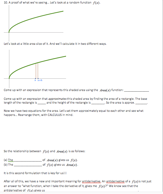
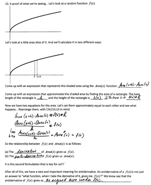
Now this page/proof should have appeared super familiar to my kids. We actually had made this exact same argument earlier when seeing the derivative of the volume of the sphere is the surface area of the sphere, and when seeing the derivative of the area of a circle is the circumference of the circle (see post here). Although this proof did require us to work together as a class with a bit more handholding than I would have liked, it went pretty well.

And with that, I can put this three part beast to bed. If nothing else, this series just reminds me how much I really think about how students build and construct knowledge. It is something that I think about so naturally when designing new materials, but to explain all that thinking and how it unfolds in the classroom takes way more words than I anticpated! No more three part blog post series for a while!

Fin.

In my last post, I outlined the road trip scenario I used to prime kids to think about areas under curves. It had nothing to do with anti-derivatives. And that’s important to keep in mind. This post is going to try to outline how we made the intellectual leap from areas under curves to anti-derivatives. [Update: I wrote this during 40 minutes of free time I had in school today where I didn’t want to do other things I was supposed to be doing. So I didn’t get to writing the part of the lesson where we make The Leap. This post ends where we’re literally all primed to make the leap. But indeed! I will make the leap with you! But in Part III. Which will be written. Soon. I hope.]

The road trip introduced this idea that kids can approximate how far someone traveled using a left-right-midpoint Riemann Sum approximation (we did not give it that name…). It arose naturally from the roadtrip scenario.

We also made the conclusion that if we had more data, we could get a better approximation for how far someone traveled. To remind you, we started with this data:

and then we got more data:

That’s going to be our transition. We are now going to give infinite velocity data! [1]

Wonderfully, kids had no problem with doing this. The reason I highlighted question 1c is because I was very intentional about including that question. When students graphed 1e, they often would draw:

I didn’t correct anyone while they were working. And it was nice to hear a few groups have the requisite conversation about why we needed to connect the points. Afterwards, when we debriefed as a whole, this was something I highlighted. We knew the position at every moment in time, including at t=2.31 (as asked in 1c).

Kids continued on with Questions 2, 3, and 4. They flew through these, actually.

These were golden. Let me say that again: these were golden. [2] It was amazing to watch kids:

• Parse the connection between velocity graphs and position graphs
• Understand the idea of negative velocity
• Think about the fact that we have to specify an initial position in order to create a position graph
• Draw a connection between motion on a number line and a graph of position v. time
• Understand what distance and displacement are, and see the difference between the two

Seriously, just watching kids work through these problems was… well, I’ll just say this feels like something I’m super proud of creating. It didn’t take much time to do but gave us so much fodder.

We didn’t need a lot of time to debrief these four questions. I had students highlight a few things, and I made sure we brought up the fact that we were drawing line segments for the position graphs, and not something curvy. Because constant velocity means position is changing at a constant rate, it’s linear. So for example, the position graph for 3c would look like what I have below. It isn’t a parabola.

But there was one huge thing we had to go over. With the roadtrip, we drew a connection between area and how far someone went. Most kids, as they were doing these problems, didn’t think about area. I wanted kids to think about area. So in our debrief, I explicitly asked them what our huge insight from the roadtrip was (area as distance travelled!), and if we could apply it to one of the problems.

So first I went back to question 2c. And I asked students how they calculated their answer:

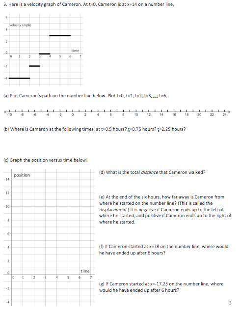
Kids said she went backwards a total of 24 units. So they did . And then I explicitly had them draw the connection to what we did with the roadtrip. This is when we talked about it being area, but “signed” to represent the backwardsness.

To be clear, some students had already been thinking in this way (about area/signed area) when working on these problems. But most hadn’t been, so we had to bring that idea to the forefront.

Then I had a student talk through Question 3 with areas in mind:

And finally, I asked groups to discuss how we could understand distance and displacement from the velocity graph.

 

 

There is one more part to this packet I had my kids work on that I will outline in my next blogpost in the series! But here’s an editable .docx of the file I made [2018-05-02 Velocity Graphs]. And here’s the document to view here:

Stay tuned for Part III.

 

[1] Both @calcdave and I stumbled upon the same approach for this!

[2] The only note is that a few students didn’t realize the time interval was 1/2 hour for Question 4. And it involves a fair amount of calculation.

 

An Important Prelude: On one of the early days in my calculus class, I have groups imagine a roadtrip. It’s one of the very best things I do, because it problematizes the idea of how something can be going at a particular speed at a moment in time. Like a speed involves a rate of change of position in a time interval, but we don’t have a time interval at a moment in time. So saying something like “we were going at 58mph at 2:03pm” suddenly goes from a statement kids accept to a problematic statement. And at that moment, we’re ready for calculus.

Setting the Stage Now: In calculus, I had gotten my kids to take tons of derivatives, and then taught them about antiderivatives and how to take them. But of course the whole time they were doing antiderivatives, they were asking “but why are we doing this?” I got this question a few times, but I just said “you’ll see very soon… probably next week… I just want to get some of this algebraic thinking out of the way so we can focus on concepts.” [1]

The Problem: I looked back at what I’ve done in the past about how to draw the connection between the antiderivative and signed areas together, and had a bunch of pretty terrible methods. I didn’t like any of them. So I put out a call on twitter while brainstorming myself. [2] I got a ton of responses, three of which stood out to me. The first one is something I kinda did at the start of the year already (before we did any calculus), so I’m excited for when my kids see the connection…

The second came was from the appropriately named @calcdave:

What’s incredible is that when I tweeted out asking for help, I had already started brainstorming … and it was so amazing that we had such similar ideas that I had to take a photo of my scratch work to send David:

 

I also got a DM from Brett Parker (@parkermathed) with a screenshot of how he digs into the idea. And what was his idea?

Yup. Driving in a car. Which of course got me thinking of the start of the year when I basically transitioned to derivatives using a road trip.

What I did: Part I

So I told kids we were going to put a pin in anti-derivatives for a short while to go on a short detour. And I used Brett’s setup, but changed it to be a followup from the roadtrip we had talked about earlier this year. We read the setup together, and then I gave each group a few minutes to talk about part (a).

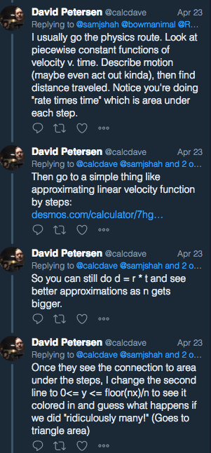
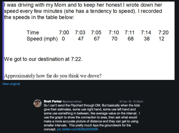
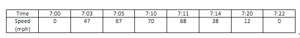
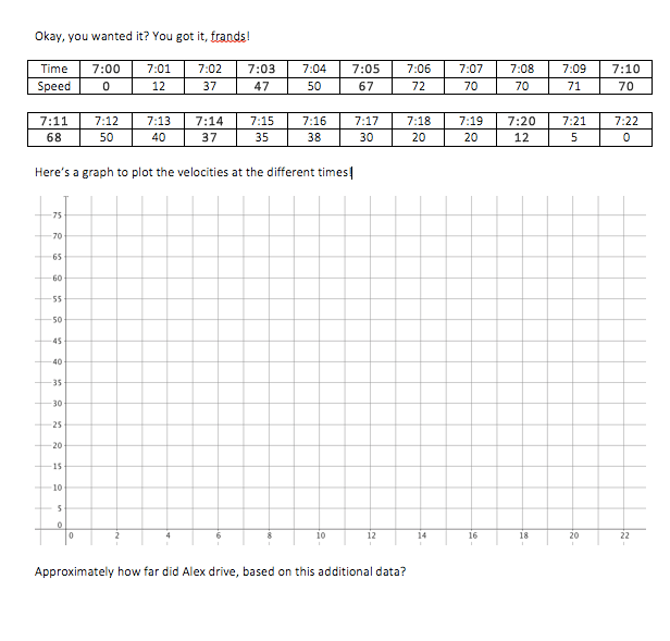
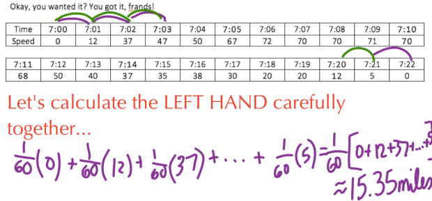
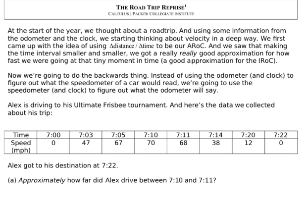
Surprisingly, this was not an easy question for kids. Many didn’t instantly think distance=(rate)(time). Additionally they didn’t know what assumption to make about the speed for the minute that passed between 7:10 and 7:11. I emphasized the approximate part of the question, and really told kids they would need to make an assumption.

When we debriefed, most kids suggested Alex was probably driving 69mph for the minute, so they did .

Some suggested he was maybe going 70mph for most of the minute, so they suggested . And with that, I suggested that maybe he was going 68mph for most of the minute… We did the calculations for all three and saw they were pretty similar.

(We also had discussed that in that minute, perhaps Alex started at 70mph, went to 100mph, and then slowed down to 68mph… We just didn’t know. So we were making and using an assumption, but one that is pretty reasonable.)

Then kids in their groups went to the next three parts. And each group was assigned an assumption: average speed, left hand speed, or right hand speed.

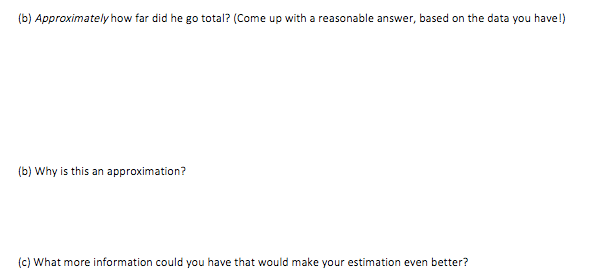
The only errors I saw kids make in part (b) was not taking the different time intervals into account. Since we did one example which had a time interval of hour, some groups were using that time interval for everything. But pretty rapidly most kids got there.

In our debrief, I wrote out the calculation kids did for the left hand assumption, and then asked students what I would have to change to do the calculation for the right hand assumption. (That was written in yellow.) This question was a key question to ensure kids understood the difference.

Then we talked why this was an approximation? (We had to make assumptions about the speed of the car at all the times inbetween the times we were given.) And then kids said that to get a more accurate distance for Alex, we’d need more data.

And that’s precisely what they got when they flipped the sheet over.

I assigned some groups the left hand assumption, and some groups the right hand assumption. I thought with so many data points, kids would be like “argh! I have to do all these calculations!” But no, there were no audible groans (I don’t think…) And they plotted the points and then did the calculations. I told kids to write out all their calculations instead of just saying how far Alex drove in the first minute, the second minute, the third minute, etc. No everyone listened. Shame. They lost out. Because when we debriefed, we saw:

Yup. The fact we could factor out the 1/60th is key. It made this all go so much faster. Only a few kids noticed that when doing the calculations. And then we compared that with the right hand assumption:

The same answer! Why? Kids saw that the sum inside the brakets (after factoring out the 1/60) would be the same because the starting speed and ending speed were both the same.

So we’re done, right? NO. We had two more moves to make.

First, we looked at the graph.

And I asked: “if we were doing the left hand assumption, what would our velocity graph look like?” And we concluded that for each 1 minute interval, Alex was driving at a constant rate. So it would look like this:

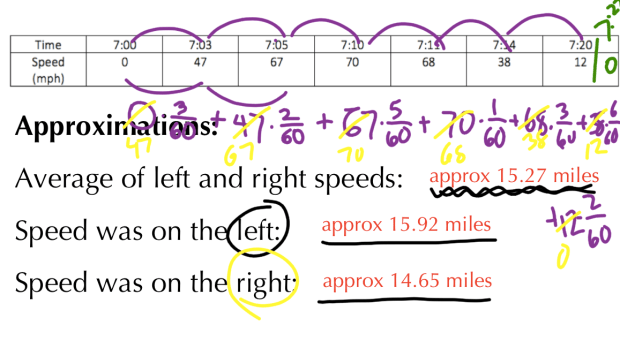
Second, I asked: Between 7:05 and 7:06, how much are we assuming Alex went? (Kids answered ) Here’s where I did some talking. I could probably have asked kids to think geometrically and had them come up with this, but I was running out of time.

I said: “where do we see 67 represented on this graph?” (Kids said the height of the velocity graph from 7:05 to 7:06.) I then said: “where do we see the on this graph?” (Kids said the 1 minute length.) So I drew a rectangle. Slowly. And then shaded it in. Slowly. And turned around. Slowly.

Yes. Audible gasps from many. I then said: “What about 7:04 to 7:05? What was our calculation for the distance Alex traveled?” And after a few more, we saw:

Kids saw. Heck yeah. They got that the approximate distance that Alex traveled was algebraically calculated in one way. And then they saw that number had a graphical representation. It was awesome.

I left by showing the original velocity points graphed. Reminded them of our left hand assumption, and that it was just an assumption, though a pretty good one. And then I drew the curve below. And dropped the microphonic device and left.

 

All in all, this was a pretty detailed blow-by-blow. And since I did it in two different classes, and things unfolded slightly differently in each, this is an amalgam of what happened. But it’s a pretty solid recap of the story I wanted to tell and how it was told. (And it’s a testament to the help of my (twitter) frands.) Most of the time, students were working. But a lot of great conversations happened as a whole class. It is a long post, but the question we worked on was only one page [editable version to download: 2018-04-30 A Road Trip Reprise] And it probably only took 20 minutes total from start to finish. A really exciting 20 minutes for me.

Stay tuned for how I used the idea that @calcdave and I both stumbled upon to make the connection between area and anti-derivatives. Right now kids have seen that there is a connection between area under a velocity curve and the distance someone has traveled. There is still no connection to anti-derivatives. That’s coming up.

[1] To be honest, I made the decision years ago to do tons of antiderivatives before introducing the integral. I wanted all the algebraic work done and solid before we introduced the concept of the integral. I didn’t want kids messing with the idea of signed area, new notation, and tough antiderivatives all at the same time. I still kind of think this is the right decision, but some doubts have crept in. I just really hate when I have to say “you’ll see why… promise…”

[2] Apparently I asked this on my blog ages ago in 2009.

Yeah, so the title of the post says it all. I am teaching a standard calculus course, and I wanted my kids to see why this beautiful thing holds true.

It’s not a coincidence. And in fact, a circle also has a nice property: the derivative of the area of a circle () gives you the circumference of the circle (). So yesterday I decided I wanted to come up with a short investigation that at least exposes my kids to this idea.

After working for around 90 minutes this morning, I ended up with a packet, and these things on my desk which I’m going to use for illustrations (blocks, dumdums, and tape):

UPDATE: I was shopping yesterday and found these gems. YAAAS!

I’ll post the packet I whipped up below. It goes through the standard argument, so in that way it’s nothing special. But in the past when I taught the course, I used to just kinda stand up at the board and give a 5 minute explanation. But I wasn’t sure who was really grokking it, and I was doing too much handwaving.

The big picture trajectory:

*At the start of class, but way before doing this activity, I’m going to have kids recall what a derivative is graphically (the slope of a tangent line), and then how we approximated it before we used limits (the slope between two points close to each other). And from that, I’m going to remind kids of the formal definition of the derivative:

* I may also start class with this problem, suggested to me on twitter by Joey Kelly (@joeykelly89). It’s a classic problem that was featured on xkcd, but oh so unintuitive and surprising!:

*Way later in class, I will transition to this activity. The first idea is to get kids to see the connection between the volume of a sphere and the surface area of a sphere. And then again for the area of a circle and the circumference of a circle.

*Then I try to get kids to understand what’s going on with the sphere first… followed by the circle.

*Then I show kids the “better explained” explanation. Why? Because at this point, kids are spending a lot of time thinking about the algebra, and I’m afraid they might have lost the bigger picture. The algebra focuses on one “shell” of the sphere, or one “ring” of the circle. But how does it all fit together? [@calcdave sent me this video, which I’d seen before but forgot about, which has the same argument… this is where the licorice wheels above come into play.]

*Finally, I problematize what they’ve learned. I have them mistakenly make a conjecture that the derivative of the volume of a cube is going to be the surface area of the cube, and the derivative of the area of a square is going to be the perimeter of the square. But quickly kids will see that isn’t quite true. So they have to tease out what’s happening.

My document/investigation [docx version to download/edit]:

My solutions:

I haven’t taught this yet. So it could be a complete disaster. I don’t have a sense of timing. I don’t know how much of this is me and how much will be them. I am just hoping tomorrow isn’t a disaster! Fingers crossed!

This is going to be a half-formed post. I wanted to get a conceptual way for kids to grok why the chain rule works in calculus. But without doing too much handwaving. And I wanted something visual.

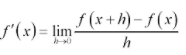
The hard part is: if we have a function , we can approximate the derivative at a particular point by doing the following.

Find  two points close to each other, like and .

Find the slope between those two points: .

There we go. An approximation for the derivative! (We can use limits to write the exact expression for the derivative if we want.)

But that doesn’t help us understand that on any level. They seem disconnected!

But I’m on my way there. I’m following things in this way:

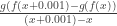
Check out this thing I whipped up after school today. The diagram on top does and the diagram on the bottom does . The diagram on the right does both. It shows how two initial inputs (in this case, 3 and 3.001) change as they go through the functions f and g.

At the very bottom, you see the heart of this. It has

And then I thought: okay, this is getting me somewhere, but it’s to abstract. So I went more concrete. So I started thinking of something physical. So I went to how maybe someone is heating something up, and in three seconds, the temperature rises dramatically. The temperature measurements are made in Farenheit, but you are a true scientist at heart and want to see how the temperature changed in Celcius.

I love this. I’m proud of this page.

And then of course when I got home, I wanted to see this process visualized, so I hopped on Geogebra and had fun creating this applet (click here or on the image below to go to the applet). These sorts of input-output diagrams going from numberline to numberline are called dynagraphs. You can change the two functions, and you can drag the two initial points on the left around. (The scale of the middle and right bar change automatically with new functions you type! Fancy!)

And of course after doing all this, I remembered watching a video that Jim Fowler made on the chain rule for his online calculus course, and yes, all my thinking is pretty much recapturing his progression.

This, to be clear, is about the fourth idea I’ve had as I’ve been thinking about how to conceptually get at the chain rule for my kids. The other ideas weren’t bad! I just didn’t have time to blog about them, but I also abandoned them because they still felt too tough for my kids. But I think this approach has some promise. It’s definitely not there yet, and I don’t know if I’ll have time to get there this year (so I might have to work on it for next year). But I know to get there I’ll have to focus on making the abstract very tangible, and not have too many logical leaps (so the chain of logic gets lost).

If I’m going to create something I’m proud of, kids are going to have to come out saying “oh, yeah… OBVIOUSLY the chain rule makes sense.” Not “Oh, I guess we did a lot of stuff and it all worked out, so it must be true.”

A blogpost of unformed thoughts, and an applet. Sorry, not sorry. This is my process!

I’m in the middle of optimization in my calculus class now. I had a “long block” (every seven school days, I see a class once for 90 minutes) and for the second half of that long block, I like to do something slightly different. Since I knew my kids hadn’t seen or done the traditional “box optimization problem” in precalculus (since I taught them last year also!), I decided to do that.

This might jog your memory if you don’t know what I’m talking about. You take a piece of paper. You cut out four squares (the same size squares) from the corners. You then fold up the four flaps and tape the box shut. There you go!

You can probably tell that the box’s volume is going to be based on the original paper you start with, and the size of the square you decide to cut out. The question is: what’s the largest volume you can get for this box. 

If you cut out a teeeny tiiiiny square, you’re going to have a very large base for the box, but almost no height. And if you cut out a giant square, you’re going to have a large height but a teeeeeeeny tiiny base. And somewhere between a teeeeeny tiny square and a giant square is going to be the perfect square to cut out which will give you the largest volume.

So the question is: given a specific piece of paper, what size square do you need to cut out to get the maximum volume.

This question has been done to death in middle school classes, in Algebra II classes, in Precalculus classes, and in Calculus classes. And I recognize that this post is just another rehashing of the same old problem. But I remember reading about a teacher who did a variation of this by including popcorn. And I wanted to do the same. No surprise, when I looked it up, it was dear Fawn. But I had such a lovely time in class today watching this unfold that I wanted to share the specific sheet I made up for kids to do this.

[2018-01-31 Popcorn Activity .docx version to download]

Teacher Moves / Outline

This activity requires students knowing and using the quadratic formula. My kids (standard level calculus) are pretty weak with algebra, so I started the class with a “do now” that had kids use the QF. So I recommend that.

Show kids the popcorn. (I had two different flavors.) Show your excitement about the activity. (I was genuinely excited!) Get this psyched. Hand out the worksheet but nothing else.

Put a three minute timer on the board. Explain the problem. Show kids a piece of cardstock with 4 squares drawn on it. Show kids a second piece of cardstock with those same four squares cut out and the flaps folded up so it looks like a box (but untaped, so you can unfold it too). Tell them the volume they create is the amount of popcorn they are going to get. And that you aren’t going to overfill their boxes — just to the brim. Tell them they have 3 minutes to work with their partner to come up with the best size square they want to cut out. And they are not allowed to do any calculations. Just visual estimation. 

At that point, give cardstock, ruler, scissors, and tape to kids. Do not let kids start until you press “GO” on the timer. Then… GO!

After three minutes, my kids were done. They measured the side length of the square they cut out and recorded it on the worksheet. They then cut and taped. They weren’t allowed to get their popcorn until they did one more thing… some math…

It was super important to me that kids didn’t measure anything, except for the side length of the square, to do these problems. Why? Because this is where I want kids to recognize the side length of the square is the height (that was obvious to all my kids), but also that when calculating the length and width, they were going to be doing 216-2x and 279-2x (where x was their side length). Only a few kids didn’t get the 2x bit (they only subtracted x), but I sent them back to their seats to rethink their length and width and they immediately got it. It was actually awesome to hear their OOOOOOHHHHH moment. But yeah, no measuring. They have to use their brainzzz to come up with the length and width with what they are given!

Only after checking their volume with me, and I said it was correct, could they fill their boxes with popcorn.

As an aside, when writing this activity, I had to decide what level of scaffolding I wanted to give for this. I decided not much. So I didn’t include any diagrams. (Well, I did put two on the very last page of the worksheet in case a kid needed some additional help. Turns out no one did.) I also initially wrote the worksheet to be in inches, but then changed to centimeters, and then after thinking a bit more, I changed to millimeters. Why? So kids don’t have to deal with fractions (inches) or decimals (centimeters), and we could keep our eye on the prize. It also made the volume huge — and so kids would have to do a little work to get the correct window when graphing.

At this point, I sent them back to their seats with popcorn in their box to then solve the general case. Close to the end of class, I posted the different volumes students got by estimation (it was a tiny class today… kids were absent or at sports).

Overall, I spent about 35 minutes on this in class. One pair finished completely. All the others are at the place where they are in the middle of the calculus work (close to being done).