In my last post, I outlined the road trip scenario I used to prime kids to think about areas under curves. It had nothing to do with anti-derivatives. And that’s important to keep in mind. This post is going to try to outline how we made the intellectual leap from areas under curves to anti-derivatives. [Update: I wrote this during 40 minutes of free time I had in school today where I didn’t want to do other things I was supposed to be doing. So I didn’t get to writing the part of the lesson where we make The Leap. This post ends where we’re literally all primed to make the leap. But indeed! I will make the leap with you! But in Part III. Which will be written. Soon. I hope.]

The road trip introduced this idea that kids can approximate how far someone traveled using a left-right-midpoint Riemann Sum approximation (we did not give it that name…). It arose naturally from the roadtrip scenario.

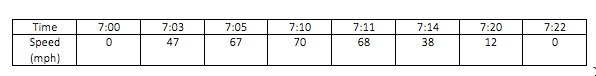
We also made the conclusion that if we had more data, we could get a better approximation for how far someone traveled. To remind you, we started with this data:

and then we got more data:

That’s going to be our transition. We are now going to give infinite velocity data! [1]

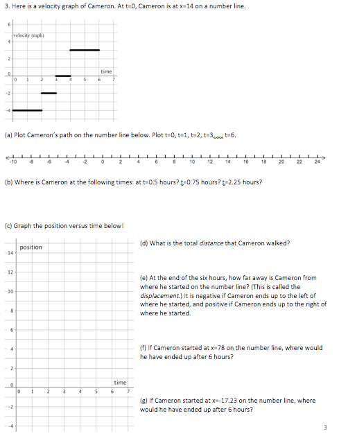
Wonderfully, kids had no problem with doing this. The reason I highlighted question 1c is because I was very intentional about including that question. When students graphed 1e, they often would draw:

I didn’t correct anyone while they were working. And it was nice to hear a few groups have the requisite conversation about why we needed to connect the points. Afterwards, when we debriefed as a whole, this was something I highlighted. We knew the position at every moment in time, including at t=2.31 (as asked in 1c).

Kids continued on with Questions 2, 3, and 4. They flew through these, actually.

These were golden. Let me say that again: these were golden. [2] It was amazing to watch kids:

• Parse the connection between velocity graphs and position graphs
• Understand the idea of negative velocity
• Think about the fact that we have to specify an initial position in order to create a position graph
• Draw a connection between motion on a number line and a graph of position v. time
• Understand what distance and displacement are, and see the difference between the two

Seriously, just watching kids work through these problems was… well, I’ll just say this feels like something I’m super proud of creating. It didn’t take much time to do but gave us so much fodder.

We didn’t need a lot of time to debrief these four questions. I had students highlight a few things, and I made sure we brought up the fact that we were drawing line segments for the position graphs, and not something curvy. Because constant velocity means position is changing at a constant rate, it’s linear. So for example, the position graph for 3c would look like what I have below. It isn’t a parabola.

But there was one huge thing we had to go over. With the roadtrip, we drew a connection between area and how far someone went. Most kids, as they were doing these problems, didn’t think about area. I wanted kids to think about area. So in our debrief, I explicitly asked them what our huge insight from the roadtrip was (area as distance travelled!), and if we could apply it to one of the problems.

So first I went back to question 2c. And I asked students how they calculated their answer:

Kids said she went backwards a total of 24 units. So they did . And then I explicitly had them draw the connection to what we did with the roadtrip. This is when we talked about it being area, but “signed” to represent the backwardsness.

To be clear, some students had already been thinking in this way (about area/signed area) when working on these problems. But most hadn’t been, so we had to bring that idea to the forefront.

Then I had a student talk through Question 3 with areas in mind:

And finally, I asked groups to discuss how we could understand distance and displacement from the velocity graph.

 

 

There is one more part to this packet I had my kids work on that I will outline in my next blogpost in the series! But here’s an editable .docx of the file I made [2018-05-02 Velocity Graphs]. And here’s the document to view here:

Stay tuned for Part III.

 

[1] Both @calcdave and I stumbled upon the same approach for this!

[2] The only note is that a few students didn’t realize the time interval was 1/2 hour for Question 4. And it involves a fair amount of calculation.