Good Math Problems

I love when kids stump me

So in multivariable calculus, it happens a lot. Most of the time, I can work things out and come back with a cogent response, and occasionally, I turn to you good folk. Today I was stumped, and then worked through it, and felt all proud of myself for about 60 minutes after I was able to figure things out. Here’s the set up and the problem:

Today, I met with a student who is working on an awesome end-of-year project on center of masses. Basically, he’s making a bunch of semi-complex foam figures (with some other materials, like wooden dowels). He’s going to multivariable calculus to find the center of mass for these figures. Then he’s going to paint them black, mark the center of mass with neon orange, and toss them in the air while video taping it.

He was inspired to do so by this video I found online:

He’s going to throw the video he makes of his own crazy figures into LoggerPro (but Tracker would work just fine) and see if he gets a parabola.

One of his objects is going to be something like 2/3 or 3/4 of a foam torus. He was having trouble finding the center of mass of it. The first thing we did was simplify the problem — changing the 3D foam figure of uniform density into a 1D bent wire of uniform density.

For the problem, we assumed 3/4 of a circular wire and we gave it a radius of 1.

Then the question was to find the center of mass for this thing. Clearly it won’t be on the wire [1], so you can think of it as such: if you wrapped the wire in super strong but super duper infinitely light saran wrap, and then you wanted to balance this wire+saran wrap figure on a pencil point, where would you place the pencil point?

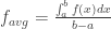
So I’ll admit that I struggled — but not as much as I anticipated. I started from first principles when solving the problem (cutting the wire into a finite number of pieces, and then making a Riemann Sum). And then this method allows me to find the center of mass no matter how much of the torus I have, whether it be 2/3 or 3/4 or e/pi.

I’m sure there’s an easy way to do this — much easier than reducing the problem to first principles and starting from scratch. But now that I have, I am pretty darn proud of myself. I think I understand the problem, now that I can look back at it, at a much deeper level. I can see symmetry arguments and how they come into play through the algebra, from working it out. I also can see how I can solve this sort of problem given any bent wire (any wire which I can describe parametrically, anyway). So yeah, I got a little bit… glowey.

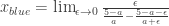
My favorite part of solving this (which involved discovering the error which confounded me for 5 minutes!) is when I ended up with:

$\int_o^{end} r\cos(\theta)\sqrt{1+\cot^2(\theta)}*-r\sin(\theta)d\theta$

Immediately I wanted to convert $\sqrt{1+\cot^2(\theta)}$ to $1/\sin(\theta)$ and have that cancel with the other $\sin(\theta)$ in the integral. That’s when I realized my huge mistake… after 5 minutes of hunting.

You can’t assume that $\sqrt{1+\cot^2(\theta)}=1/\sin(\theta)$ . In fact, it equals $1/|\sin(\theta)|$ . And this small distinction makes all the difference in the world!

No, there isn’t any advice for you, and this isn’t about things I’m doing in my class, or even me fretting about how I’m not doing an amazing job. This blog also acts as a little digital archive, and I wanted to set aside this little glowey moment.

And if you’re wondering, I’m going to let my student sweat it out, and keep on working at it, until we next meet. If he hasn’t had that moment of insight yet, I’ll help him out.

PS. If you want to work out this problem or any variation, and come up with some beautiful and elegant solution (which y’all are oh so amazing at!!!), feel free to throw your thoughts/approaches/etc. in the comments.

[1] What he’s going to do, in order to throw it, is to put two or three light toothpicks in this partial torus, with a neon orange sticker attached to the toothpicks where the center of mass is calculated to be.

Weights! Goldsmiths! Optimization!

I am in a problem solving group at my school, and I took 45 minutes of one of our sessions to lead a mock class. Not really mock, to be fair. I assumed I’d have 3 math teachers and 2 science teachers as my class, and I wanted a problem which would get them to think, work together, and also let me guide without leading (or is it lead without guiding).

The problem I chose was exactly the problem that Brent just wrote about on The Math Less Traveled: the broken weight problem.

A merchant had a forty pound measuring weight that broke into four pieces as the result of a fall. When the pieces were subsequently weighed, it was found that the weight of each piece was a whole number of pounds and that the four pieces could be used to weigh every integral weight between 1 and 40 pounds. What were the weights of the pieces? [I gave the problem with ounces.]

I have to say that I was really thrilled that I was able to get them to a solution, with very little nudging. I let them take their time. I started them out by giving them slips of paper of various sizes with corresponding weights written on them, and asked them to use those weights to be able to weigh something like 10 ozs. I helped them organize their thoughts with observations, and I helped them latch onto key ideas once they emerged. I never gave the key ideas, and I didn’t push. It was awesome to witness them work together.

It was also surprising in two other ways:

1. I had the pathway in mind that I thought they were going to take — basically a recursive approach. They did not go that way, and it was afterwards — when examining the problem once they had the solution – that they saw the recursion.

2. I had prepared two “hint cards.” They were written on origami paper and folded up — because, why not? I told ’em that if they all agreed, they could take the first hint card, and if they felt they really needed it, they could have the second hint card. They didn’t take any of ’em. I thought they would. In fact, I predicted that they would get frustrated and take the first one pretty quickly, so I put on the first hint card: “YOU CAN DO IT! Keep working at least for another 5 minutes.” It wasn’t a hint, but a “work through frustration” note. The second card had a hint leading them to recursion (saying something like “What if you only had any 2 weights… what would they be so that you can weigh the most: 1 oz? 2 ozs? 3ozs? 4 ozs? …”)

As a result of watching them operate, and places they struggled (including understanding the problem!), I wanted to challenge myself.

How could I create a formal lesson plan for this? A lesson plan that guides without leading.

Here’s my first crack at it (PDF here):

View this document on Scribd

PS. Yes, I know there’s a typo in question 1.

Solution to the “what curve is this?” problem

So a while ago I posted a problem that me and another teacher worked on in our problem solving group. We didn’t have the most elegant solution (that honor goes to Jake), But I think it is slightly qualitatively different than the solutions posed in the comments of the original post. Our solution involved systems of equations and parametric equations and L’Hopital’s rule. Yup, believe it or not, L’Hopital arose naturally in the wild, and when I was coming up with my plan of attack, I suspected it would if things were going right.

To remind you, I wanted to find the equation for this blue curve:

(If you want more details, just check out the original problem.)

So here it goes.

The crucial question we asked ourselves is: if we drew all the red lines, where would the blue line come from?

The answer, which was fundamental for our solution, was: if we drew two red lines which were infinitessimally close to each other, their intersection would give us one point on the blue curve. Think about that. That is the key insight. The rest is algebra. If we could find all these intersection points, they form the line.

So we picked two points close to each other: one with endpoints $(a,0)$ and $(0,5-a)$ and the other with endpoints $(a+\epsilon,0)$ and $(0,5-a-\epsilon)$ .

Notice that as we bring $\epsilon$ closer and closer to 0, these two lines are getting closer and closer to being identical. But right now, $\epsilon$ is just any number.

So the first line is (in slope-intercept form): $y=-\frac{5-a}{a}x+5-a$ (any of the red lines)
And the second line is: $y=-\frac{5-a-\epsilon}{a+\epsilon}x+5-a-\epsilon$ (any of the other red lines)

We want to find the point of intersection. So setting the $y$ s equal to each other and solving for $x$ , we get:

$x=\frac{\epsilon}{\frac{5-a}{a}-\frac{5-a-\epsilon}{a+\epsilon}}$

Of course now we want to see what happens to the intersection point as we bring the two lines infinitely close together. So we are going to take the limit as $\epsilon$ approaches 0.

$x_{blue}=\lim_{\epsilon \to 0} \frac{\epsilon}{\frac{5-a}{a}-\frac{5-a-\epsilon}{a+\epsilon}}$

Notice you’ll see that we get a $0/0$ form if we just plug in $\epsilon=0$ , so we must L’Hopital it!

When we do that (remember we take the derivative of the numerator and denominator with respect to $\epsilon$ ), we find that:

$x_{blue}=\frac{a^2}{5}$ .

And plugging that into our equation for the first line, we find that the $y_{blue}$ coordinate is:

$y_{blue}=\frac{(a-5)^2}{5}$

At this point, we rejoyce and do the DANCE OF JOY!

GAAAK! Almost. You silly fools. You’re like my kids, who get so proud when they do the hard part of a problem, that they forget what the question is asking and move on to the next problem. We still don’t have an equation. And what does $(x_{blue},y_{blue})$ mean anyway?

To start, that point represents the intersection point of two lines infinitesimally close to each other in our family of red lines above. But this $a$ business? It’s confusing. I like to think of it like a parameter! As I move $a$ between $0$ and $5$ , I am going to get out all the points on the blue curve.

So how do I find this curve? Exactly how I would if these were parametric equations:

$x=\frac{a^2}{5}$ and $y=\frac{(a-5)^2}{5}$ .

I take the first equation and solve it for $a$ : $a=\sqrt{5x}$ .

I then plug that value into the second equation for $y$ : $y=\frac{(\sqrt{5x}-5)^2}{5}$ .

And we’re done! We graph to confirm:

And now, indeed, we may do the dance of joy!

MEAN (grrr) value of a function!

In calculus today I was talking about how to find the average height of a function. Some kids just have a hard time understanding the concept. I always show them a few functions on certain intervals and I ask them what they think the average height would be. Just to initially test their intuition on the concept.

Some see it, and understand it; some don’t. All certainly have trouble articulating why they chose that value.

So I have two things that work for me, when explaining this. There’s some handwaving, but the focus is on the idea, and building intuition.

The first thing is we talk about how we would approximate the average temperature somewhere:

We take a bunch of temperature readings, and we add them together and divide by the number of readings.

How do you make it more accurate?

Parametrization, Parabolas, Calculus, OH MY!

Okay, so a second problem in a row! This one is a straight up calculus one, from the 2008 AP Calculus BC exam — multiple choice section. The teacher of that class asked me if I could work this problem — and I admit I struggled. She showed me her solution, and then I left thinking “it couldn’t be that hard…”

When trying to fall asleep today, I started thinking of it and I was able to solve it in a different way.

Without any more preamble, if you care to try your hand at this:

A particle is moving along the curve $y=x^2-x$ at a constant speed of $2\sqrt{10}$ . When it reaches the point $(2,2)$ , you know $\frac{dx}{dt}>0$ . Find the value of $\frac{dy}{dt}$ at that point.

As usual, feel free to throw your thoughts, solutions, etc. in the comments below, if you want. I bet for many of you this will be super easy, but for the few of you who struggle through it (sigh) like me, you might find it actually frustratingly enjoyable.

Oh, and also throw down there if you get stuck and care to see my solution… It’ll motivate me to actually type it up in a timely fashion.

A good problem solving problem

So… I am in this “problem solving” group at school, and we spent today trying to come up with a lesson centered around problem solving that we could use for one of our classes.

I’ve been really hankering to make one of these hyperboloids out of skewers:

and I thought it would be a great investigation for my multivariable class to figure out if indeed that was a hyperboloid of one sheet. I figured it would take a number of days — at least one to create one of our own, and a good number to figure out how in the world we would come up with the equation to define that beast. [1]

Of course one of the things we talked about in our problem solving group is how to bring the questions down to simpler questions — and then generalize. So I immediately thought of these drawings I spent hours of my childhood making:

[Yes, clearly my mother was happy that I found these to amuse myself with, instead of whiiiiiining “I’m so BORED… we have NOTHING to do in this house” as I did way too often.]

If you look, they define a really nice gently sloping curve.

So my question is: what is the equation (written in terms of x and y) for the curve above?

The first segment goes from (0,5) to (0,0). Then another segment might go from (0,4) to (0,1). Another segment might go from (0,3.5) to (0,1.5). (So however much down you go on the y-axis, you go that much right on the x-axis.)

I haven’t solved the harder 3-d question yet, but I had a heck of a time solving this 2-d question.

Since I had so much fun, I thought I’d share the problem with you!

I’ll post my solution later, but if you want to throw your solution down in the comments and how you came up with it (or blog about it), awesome. Just like with this “circles, circles everywhere” problem where someone posted the most elegant solution EVAR.

Riemann Sums and Error

Sometimes I wonder about my sanity. Our school gets a 2 week spring break. I decided to teach my calculus classes on the last day before break. And I meet one of them during the last period. So yeah, sanity?

As you know, I’ve been working on Riemann Sums. After calculating them by hand [worksheet here], I had my kids enter this program in their graphing calculators.

We of course talked about why the program actually gives you the Riemann Sum. I’m going to expect them to be able to answer a question on the assessment about it. All that calculator stuffs was on Thursday.

They were coming to school on Friday with this program entered on their calculator.

I got home on Thursday at 9ish pm and when weighing the options of “show Stand and Deliver” or “create a lesson plan,” I just couldn’t let go of the fact that if I waited until after spring break to capitalize on this program, the momentum would be lost. So lesson plan it was. And I whipped the lesson plan [.doc here] below in about 90 or 100 minutes.

View this document on Scribd

I told my kids that the fundamental question that we are tackling is: what is the relationship between the number of rectangles in our Riemann Sum and the error to the true value? And then we talked about what they already know … which is as the number of rectangles increase, the error decreases. So I modified our question: what is the MATHEMATICAL relationship between the number of rectangles in our Riemann Sum and the error to the true value?

We’re studying a a semi-circle of radius 2.

And so they use the program and come up with a bunch of data

And since they are interested in N and the error, they enter those values into lists in their calculator. Looking at a graph for low N values versus the error, they see this on their calculators:

So yes, they see that as N increases, the error goes down to zero. Mr. Shah’s eyes are wide open with awe.

That’s as far as we got in class on Friday. When we return from break we’re going to find a curve to fit this data. They’re going to try to fit this data to linear, exponential, logarithmic, and power functions using their calculators. It turns out that you can find a great power function to match this data. Seriously amazing. (The others don’t turn out well at all.)

That’s only for low N (from 0 to 20). Will our power function hit the N=500 point?

YEAAAAAH! This is where I started to get excited when I was creating my lesson. Because I thought that the error function would get really off so far out in the data. But heck, it’s pretty awesome that it hits at N=500.

I was curious HOW much our error function helps us with our estimation. So the last part of the activity is having students use only 75 Riemann Sums to estimate the area of the semi-circle. The error is shown below.

Not bad. But we have found a function models how much error using 75 rectangles will give us. So adding in that correction factor gives us a NEW estimation of the true area. And how much is this new estimation from the true value?

Um, using our error function as a correction factor gives us an answer that is 5 orders of magnitude better. Instead of an error of $10^{-2}$ we get an error of $10^{-7}$ .

I was really shocked and pleased by this! That’s where the lesson ends. Partly because I was too tired to make more, and partly because I want to move on in the course. I have a number of questions still lingering in my head, that I will be thinking about over break. Including why the error takes the form of a power function for this function (the semi-circle)?

Also, I still have a problem with the circularity of it all. I needed (a priori) the true area of the semi-circle to calculate the error for each N. Then we use these errors to find a curve to match the error associated with each N. This curve gives us a correction factor which gives us a better approximation to the true area. But if the point of all of this was to find the true area, we actually had to know it at the start to come up with the errors!

Some part of me wants to say that there is a good response to that. I suspect there is, and it deals with computing time. Like “say you want a good approximation. Start by assuming your true area is the Riemann Sum calculated for N=1000. Then use that to come up with the error curve. This error curve will then help you come up with a better approximation for the true area.” Or something like that. I don’t know, really. I’m just talking about nothing at the moment.

Continuous Everywhere but Differentiable Nowhere

I have no idea why I picked this blog name, but there's no turning back now