Doodling in Math

A few years ago, I blogged about this fun little doodle that students often make — and how another teacher and I found out the equation that “bounds” the figure. I honestly can’t remember if I ever posted how I got the answer. If I did and this is a repeat, apologies.

Tonight I wanted to see if I could re-derive it like I did before — and lo and behold I did. I’m curious if any of you have done it the way I did it, or if there are other ways you’ve learned to approach this problem. (There is a student who I had last year who created this amazing 3-d version of this using the edges of a cube and some string. I love the idea of asking — for this 3-d figure — what surface is generated by the intersections of these strings.)

We start out by having these lines which form a family of curves. But of course we’re not graphing all the lines. If we were, we’d get something more dense like this.

The main idea of what I’m going to do to find that curve… I’m going to pick two of those lines which are infinitely close to each other and find their point of intersection. That point of intersection will lie on the curve. (That’s the big insight in this solution.) But I’m not going to pick two specific lines — but instead keep things as general as possible. Thus when I find that point of intersection for those two lines, it will give me all the points of intersection for all the lines.

Watch.

First we pick two arbitrary lines.

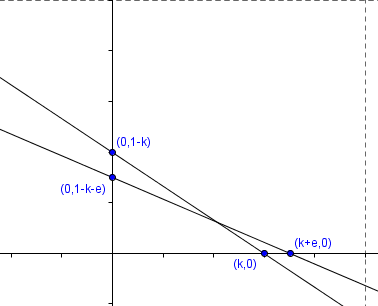
We’ll have one line move down on the y-axis $k$ units (and thus over on the x-axis $k$ units). And the second line will be moved down on the y-axis just a tiny bit more (down an additional $e$ units). Yes, we are going to have that tiny bit, that $e$ , eventually go to zero.

The two lines we have are:

$y=\frac{k-1}{k}(x-k)=\frac{k-1}{k}x-(k-1)$

$y=\frac{k+e-1}{k+e}(x-(k+e))=\frac{k+e-1}{k+e}x-(k+e-1)$

A little bit of algebra is needed to find the point of intersection. Setting the y-values equal:

$\frac{k-1}{k}x-(k-1)=\frac{k+e-1}{k+e}x-(k+e-1)$

And then doing some basic algebra:

$k^2+ke=x$

Now solving for $y$ we get:

$y=\frac{k-1}{k}(k)(k+e)-(k-1)$

$y=k^2+ke-2k-e+1$

So the point of intersection is:

$(k^2+ke, k^2+ke-2k-e+1)$

Here’s the kicker… Remember we wanted the two lines to be infinitely close together, right? So that means that we want $e$ to go to zero. Thus, our point of intersection of these infinitely close lines will be:

$(k^2, k^2-2k+1)$ or $(k^2,(k-1)^2)$ .

Beautiful! And recall that we picked the lines arbitrarily. By varying $0\leq k \leq 1$ and plotting $(k^2,(k-1)^2)$ , we can get any two lines on our doodle.

But I want an equation.

Simple. We know that $x=k^2$ . Thus $x=\sqrt{k}$ .*

Since $y=(k-1)^2$ , we have $y=(\sqrt{x}-1)^2$

Let’s graph it to check.

Huzzah!!! And we’re done!

I wonder if I can do something similar with this cardioid:

I think I must (for funsies) do some investigation of “envelopes” this summer. I mean, Tina at Drawing on Math even introduces conics with these envelopes!

An extension for you. Do something with this 3d string-art.

*Of course you might be wondering why I don’t say $x=\pm \sqrt{k}$ . Since $k$ is between 0 and 1, we know that $x$ must be positive.

8 comments

Now I can’t remember how I did it. I do remember coming to the form sqrt(x) + sqrt(y) = 1, though.

Lovely exposition, Sam!
I’ll leave these two Daily Desmos challenges here in case they’re useful to someone:
http://dailydesmos.com/2013/10/16/daily-desmos-218b-basic/
http://dailydesmos.com/2013/10/16/daily-desmos-218a-advanced/

I love this stuff. A couple related GeoGebra sketches: http://www.geogebratube.org/material/show/id/46238 for string art on curves, http://www.geogebratube.org/material/show/id/43283 for piecewise linear.

Hello Sam
What you have done for the k and 1 – k example is exactly the general approach, which is much easier until the last step. Here goes :-
Straight line parameterized with a is y = f(a)x + g(a)
“Next ” line is y = f(a + h)x + g(a + h)
Start solving for x and y by eliminating the y
0 = (f(a + h) – f(a))x + g(a + h) – g(a)
Divide by h for h0
(f(a + h) – f(a)) + g(a + h) – g(a)
0 = —————- x + ——————-
h h
or, since this will be messed up,
0 = (f(a + h) – f(a))/h * x + (g(a + h) – g(a))/h
Letting h go to zero then gives
0 = f'(a)*x + g'(a)
So far, very neat, but the messy bit is now eliminating a from this and the original equation.

A fairly simple one is y = ax + 1/a
The cardioid will probably drive you insane!
Howard

Again!
Your y = root x -1 all squared is a parabola

Cool! Thank you! I love that this involves derivatives!

cos(a) x + sin(a) y = 1
and/or
sqrt(1-k) x + sqrt(k) y = 1
also work well with this method (at least once you’ve proved the general derivative result Howard Phillips gave above).

In terms of constructions, if you draw lines where the *product* of their intercepts is constant (rather than the *sum*), you also get a nice picture…

Well! You have shared very helpful stuff. I really like your collection and i appreciated your way to describing your article with the help of different pictures. You have done really good job. I would like to say Thanks for sharing such a nice collection. I have found helpful collection regarding Math from a website which i like to share this website.
http://www.ipracticemath.com/math-practice

Continuous Everywhere but Differentiable Nowhere

I have no idea why I picked this blog name, but there's no turning back now

Doodling in Math

8 comments

Leave a Reply Cancel reply

Share this:

Like this:

Related

8 comments

Leave a Reply Cancel reply