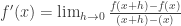
The Formal Definition of the Derivative, or Why Holes Matter

Lucky you! Two calculus posts in one day. Mainly because I don’t want some of these ideas to disappear in my hiatus from teaching it. This one deals with our favorite topic: the formal definition of the derivative.

$\lim_{h \rightarrow 0}\frac{f(x+h)-f(x)}{(x+h)-(x)}$

I see that expression and my mind goes to the following places:

Doing a bunch of tedious algebraic calculations for a particular function in order to find the derivative.
I “see” in the expression the slope of two points close together.
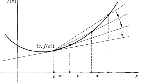
I envision the following image, showing a secant line turning into a tangent line

And I think for many teachers and most calculus students, they think something similar.

However I asked my (non-AP) calculus kids what the $h$ stood for. Out of two sections of kids, I think only one or two kids got it with minimal prompting. (Eventually I worked on getting the rest to understand, and I think I did a decent job.) I dare you to ask your kids and see what you get as a response.

What I suspect is that kids get told the meaning of $\lim_{h \rightarrow 0}\frac{f(x+h)-f(x)}{(x+h)-(x)}$ and it gets drilled into their heads that they might not fully understand what algebraically is going on with it.

It was only a few years ago that I came to the conclusion that even I myself didn’t understand it. And when I finally thought it all through, I came to the conclusion that all of differential calculus is based on the question: how do you find the height of a hole? I started seeing holes as the lynchpin to a conceptual understanding of derivatives. I never got to fully exploit this idea in my classes, but I did start doing it. It felt good to dig deep.

The big thing I realized is that I rarely looked at the formal definition of the derivative as an equation. I almost always looked at it as an expression. But if it’s an equation…

$f'(x)=\lim_{h \rightarrow 0}\frac{f(x+h)-f(x)}{(x+h)-(x)}$

… what is it an equation of? An equation with a limit as part of it?! Let’s ignore the limit for now.

Without the limit, we have an average rate of change function, between $(x,f(x))$ and $(x+h,f(x+h))$ . And since we have removed the limit, we really have a function of two variables.

$AvgRateOfChange(x,h)=\frac{f(x+h)-f(x)}{(x+h)-(x)}$

We feed an $x$ and $h$ into the function, and we get an output of a slope! It’s the slope between $(x,f(x))$ and $(x+h,f(x+h))$ !

Let’s get concrete. Check out this applet (click the image to have it open up):

On the left is the original function. We are going to calculate the “average rate of change function” with an x-input of 1.64 (the x-value the applet opens up with).We are now going to vary h and see what our average rate of change function looks like: 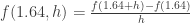$f(1.64,h)=\frac{f(1.64+h)-f(1.64)}{h}$ . That’s what the yellow point is.

Before varying h, notice in the image when h is a little above 2, the yellow “Average Rate of Change” dot is negative. That’s because the slope of the secant line between the original point $(1.64, f(1.64))$ and a second point on the function that is a little over 2 units to the right is negative. (Look at the secant line on the graph on the left!)

Now let’s change h. Drag the point on the right graph that says “h value.” As you drag it, you’ll see the second point on the function move, and also the yellow point will change with the corresponding new slope. As you drag h, you’re populating points on the right hand graph. What’s being drawn on the right hand graph is the average rate of change graph for all these various distances h!

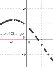
Here’s an image of what it looks like after you drag h for a bit.

Notice now when our h-value is almost -3 (so the second point is 3 horizontal units left of the original point of interest), we have a positive slope for the secant line… a positive average rate of change.

The left graph is an $x-f(x)$ graph (those are the axes). The right graph is a $h-AvgRateOfChange$ graph (those are the axes).

Okay okay, this is all well and dandy. But who cares?

I CARE!

We may have generated an average rate of change function, but we wanted a derivative function. That is when h approaches 0. We want to examine our average rate of change graph near where h is 0. Recall the horizontal axis is the h-axis on the right graph. So when h is close to 0, we’re looking at the the vertical axis… Let’s look…

Oh dear missing points! Why? Let’s drag the h value to exactly h=0.

The yellow average rate of change point disappeared. And it says the average rate of change is undefined! 0/0. We have a hole! Why?

(When h=0 exactly, our average rate of change function is: $\frac{f(x+0)-f(x)}{(x+0)-x}$ which is 0/0. YIKES!

But the height of the hole is precisely the value of the derivative. Because remember the derivative is what happens as h gets super duper infinitely close to 0.

We can drag h to be close to 0. Here h is 0.02.

But that is not infinitely close. So this is a good approximation. But it isn’t perfect.

And this is why I have concluded that all of differential calculus actually reduces to the problem of finding the height of a hole.

Here are three different average rate of change applets that you might find fun to play with:

one (this is the one above) two three

In short (now that you’ve made it this far):

Look at the formal definition of the derivative as an equation, not an expression. It yields a function.
What kind of function does it indicate? An average rate of change function. And in fact, thinking deeply, it actually forces you to create a function with two inputs: an x-value and an h-value.
Now to make it a derivative, and not an average rate of change, you need to bring h close to 0.
As you do this, you will see you create a new function, but with a hole at h=0.
It is the height of this hole that is the derivative.

PS. A random thought… This could be useful in a multivariable calculus course. Let’s look at the average rate of change function for $f(x)=x^2$ :

$AverageRateofChange(x,h)=\frac{(x+h)^2-x^2}{h}$

Let’s convert this to a more traditional form:

$z=\frac{(x+y)^2-x^2}{y}$

Now we have a function of two variables. We want to find what happens as h (I mean y) gets closer and closer to 0 for a given x-value. So to do this, we can just visually look at what happens to the function near y=0. Even though the function will be undefined at all points where y=0, visually the intersection of the plane y=0 and the average rate of function should carve out the derivative function.

If this doesn’t make sense, I did some quick graphs on WinPlot…

This is for $f(x)=x^2$ . And I graphed the plane where y=0. We should get the intersection to look like the line $f'(x)=2x$ .

Yup. Cool.

I did it for $f(x)=\sin(x)$ also… The intersection should look like $f'(x)=\cos(x)$ .

6 comments

howardat58 says:

August 13, 2014 at 3:31 am

Why, oh why, are teachers burdening the kids with the formal definition of the derivative if they (the teachers) haven’t got the gumption to show that the ratio IS the slope of the secant at all points other than the h=0 point.
What you have done is what I would do as an introduction to calculus, via slope of the line joining the x point to another point on the curve.
It can be done with a calculator.
Also, it is quite easy to show that the slope function for x^2 is 2x without ANY talk about limits.

1. rprsns says:
  
  August 14, 2014 at 6:32 pm
  
  I totally agree with you, howardat58. Could you expand on your calculator thought and give a bit more detail about your last line? My curiosity has been piqued.
  
cheesemonkeysf says:

August 13, 2014 at 4:11 am

As soon as I saw the notice appear in my In Box, my immediate uncensored reaction was, “Wow, what a show-off, doing TWO calculus blog posts in one day.” But then I saw that you acknowledged your overachievement with a very respectable reason, and so I felt suitably ashamed of myself. :)

– Elizabeth (@cheesemonkeysf)

mrdardy says:

August 14, 2014 at 10:27 am

Quick thought on notation. Early in my career when I was a bit more stubborn I chose not to use h in the definition of the derivative instead using a delta x there. The notation got very ugly as we were expanding and finding the derivative by hand (I’m showing my age here, I fear) and the students certainly did not like keeping track of squares and cubes of delta x. Looking back, I suspect that they might have had a better idea of what the definition of the derivative was saying since that delta x has a more inherent meaning than the h does. Just wondering…

@MrLeiss says:

August 15, 2014 at 4:58 pm

I really wasn’t sure what you meant by the height of the hole until looking at the applet you created. The xyz graphs helped too. Very neat way of thinking in a different (for me) way about derivatives, slopes, functions as being part of the same world.

It has taken me a long time to care at all about the motivation for derivatives; since in most cases taking them (using the patterns relating to polynomials, trig, etc) is easy and powerful. I’m glad it’s finally sinking in for me (same thing with sums for integrals). Thanks for sharing this stuff and pushing things around and together in my brain!

John Palkovic says:

August 16, 2014 at 4:06 pm

There’s more than one way to do it in math.

There is a rigorous foundation for the calculus that was formulated by Abraham Robinson in 1960 that does not use limits. It uses “infinitesimals” instead. This was Newton’s approach to formulating the calculus. Newton did not use limits, yet students are often told that he invented calculus.

An infinitesimal is a quantity so small that although it is not zero, its square and higher powers are zero. Before you reject this notion, remember your math history. There was a time when no one knew of the square root of -1, yet you have probably heard of it, right? Here’s a reference, with the formal, rigorous definition of infinitesimals

http://www.sjsu.edu/faculty/watkins/infincalc.htm

or read about it in H. Jerome Keisler’s book, which is online:

http://www.math.wisc.edu/~keisler/calc.html