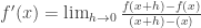
Lucky you! Two calculus posts in one day. Mainly because I don’t want some of these ideas to disappear in my hiatus from teaching it. This one deals with our favorite topic: the formal definition of the derivative.
I see that expression and my mind goes to the following places:
- Doing a bunch of tedious algebraic calculations for a particular function in order to find the derivative.
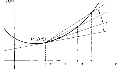
- I “see” in the expression the slope of two points close together.
- I envision the following image, showing a secant line turning into a tangent line

And I think for many teachers and most calculus students, they think something similar.
However I asked my (non-AP) calculus kids what the 
What I suspect is that kids get told the meaning of 
It was only a few years ago that I came to the conclusion that even I myself didn’t understand it. And when I finally thought it all through, I came to the conclusion that all of differential calculus is based on the question: how do you find the height of a hole? I started seeing holes as the lynchpin to a conceptual understanding of derivatives. I never got to fully exploit this idea in my classes, but I did start doing it. It felt good to dig deep.
The big thing I realized is that I rarely looked at the formal definition of the derivative as an equation. I almost always looked at it as an expression. But if it’s an equation…
… what is it an equation of? An equation with a limit as part of it?! Let’s ignore the limit for now.
Without the limit, we have an average rate of change function, between 


We feed an 
Let’s get concrete. Check out this applet (click the image to have it open up):

On the left is the original function. We are going to calculate the “average rate of change function” with an x-input of 1.64 (the x-value the applet opens up with).We are now going to vary h and see what our average rate of change function looks like: 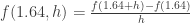
Before varying h, notice in the image when h is a little above 2, the yellow “Average Rate of Change” dot is negative. That’s because the slope of the secant line between the original point 
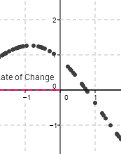
Now let’s change h. Drag the point on the right graph that says “h value.” As you drag it, you’ll see the second point on the function move, and also the yellow point will change with the corresponding new slope. As you drag h, you’re populating points on the right hand graph. What’s being drawn on the right hand graph is the average rate of change graph for all these various distances h!
Here’s an image of what it looks like after you drag h for a bit.

Notice now when our h-value is almost -3 (so the second point is 3 horizontal units left of the original point of interest), we have a positive slope for the secant line… a positive average rate of change.
The left graph is an 
Okay okay, this is all well and dandy. But who cares?
I CARE!
We may have generated an average rate of change function, but we wanted a derivative function. That is when h approaches 0. We want to examine our average rate of change graph near where h is 0. Recall the horizontal axis is the h-axis on the right graph. So when h is close to 0, we’re looking at the the vertical axis… Let’s look…
 Oh dear missing points! Why? Let’s drag the h value to exactly h=0.

The yellow average rate of change point disappeared. And it says the average rate of change is undefined! 0/0. We have a hole! Why?
(When h=0 exactly, our average rate of change function is: 
But the height of the hole is precisely the value of the derivative. Because remember the derivative is what happens as h gets super duper infinitely close to 0.
We can drag h to be close to 0. Here h is 0.02. 
But that is not infinitely close. So this is a good approximation. But it isn’t perfect.
And this is why I have concluded that all of differential calculus actually reduces to the problem of finding the height of a hole.
Here are three different average rate of change applets that you might find fun to play with:
one (this is the one above) two three
In short (now that you’ve made it this far):
- Look at the formal definition of the derivative as an equation, not an expression. It yields a function.
- What kind of function does it indicate? An average rate of change function. And in fact, thinking deeply, it actually forces you to create a function with two inputs: an x-value and an h-value.
- Now to make it a derivative, and not an average rate of change, you need to bring h close to 0.
- As you do this, you will see you create a new function, but with a hole at h=0.
- It is the height of this hole that is the derivative.
PS. A random thought… This could be useful in a multivariable calculus course. Let’s look at the average rate of change function for 

Let’s convert this to a more traditional form:

Now we have a function of two variables. We want to find what happens as h (I mean y) gets closer and closer to 0 for a given x-value. So to do this, we can just visually look at what happens to the function near y=0. Even though the function will be undefined at all points where y=0, visually the intersection of the plane y=0 and the average rate of function should carve out the derivative function.
If this doesn’t make sense, I did some quick graphs on WinPlot…
This is for 

Yup. Cool.
I did it for 


 s into
  s and
s and  s. And viola! It works out. It’s very powerful. And it’s procedural. And kids have throughout the years learned this “substitution”-y thing works [1]. So kids tend to like it.
 plane.
 ?” for example.
 and
and  .
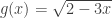
. is secretly
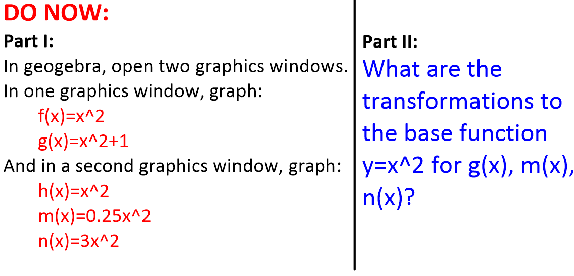
  which has undergone a vertical stretch of 2, a horizontal shrink of 1/5, and has been moved up 1.
 . It is approximately
  .
.


 .
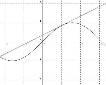
. , which is simply the slope of the tangent line of
  at
at  .
. and
and  are composed to get our final function, we can compose the tangent lines to these two functions to get the final tangent line at
  (I’m not showing the work, but you can trust me that it’s true, or work it out yourself.)
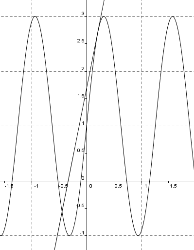
 which really means that we’re taking the square root of 9. We we want the tangent line to
  . That turns out to be (again, trust me?):
  .
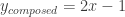
.![y_{composed}=\frac{1}{6}[12x-15]+\frac{3}{2}](https://s0.wp.com/latex.php?latex=y_%7Bcomposed%7D%3D%5Cfrac%7B1%7D%7B6%7D%5B12x-15%5D%2B%5Cfrac%7B3%7D%7B2%7D&bg=ffffff&fg=333333&s=0&c=20201002)
![yup]](https://samjshah.com/wp-content/uploads/2013/12/yup.png)
 where we can clearly remember which one is the inner and which one is the outer functions. Let’s pick a point
  where we want to find the derivative.
 at
at 

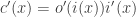
![y_{composed}=o'(i(x_0))[i'(x_0)x+blah1]+blah2](https://s0.wp.com/latex.php?latex=y_%7Bcomposed%7D%3Do%27%28i%28x_0%29%29%5Bi%27%28x_0%29x%2Bblah1%5D%2Bblah2&bg=ffffff&fg=333333&s=0&c=20201002)

 .
.
 . Why? Because even though I could teach them that (and I have in the past), I would rather spend my time doing less work on moving through algebraic hoops, and more work on deep conceptual understanding.
 as
as  ?
? and
and 
 wasn’t a good second point, and how
  also wasn’t a good second point. But if they trusted me on using this variable thingie, they will see how our problems would be resolved.
 , it means what blah gets infinitely close to if


 . Thus we can say:
 gets infinitely close to 6.
 at
at 
 at
at 
 at
at  (why it is allowed to be “cancelled” out), and then what happens as
  and they will be able to. They will see there is a jump at
  . I don’t need more than that.
 , then

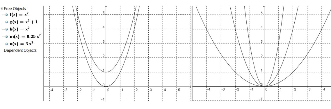
 . When the function moved up one unit, we see the tangent line simply moved up one unit too.
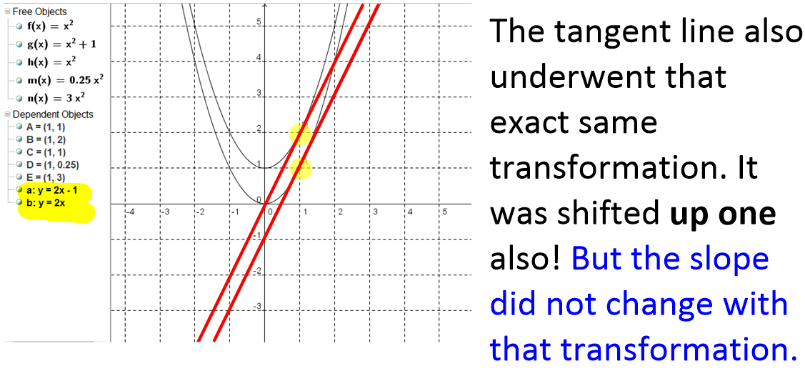
 (because you are multiplying all y-coordinates by 1/4. And that simplifies to
  . Yup, that’s what Geogebra said the equation of the tangent line was!
 . And yup, that’s what Geogebra said the equation of the tangent line was.
 , so I show them what Wolfram Alpha gives them.
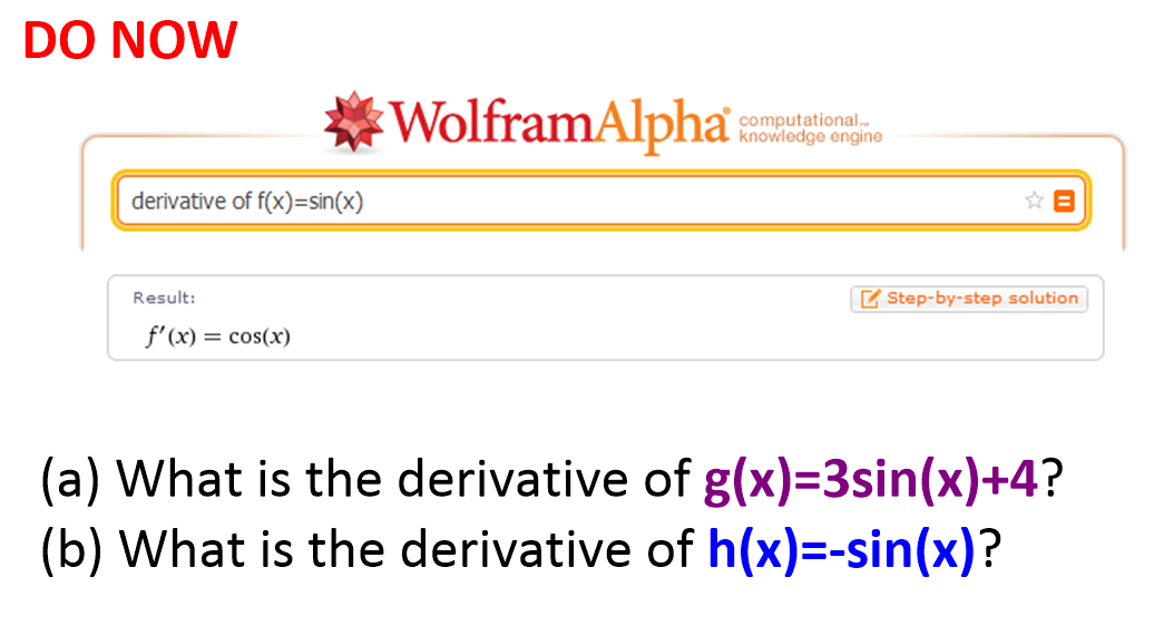
 and for (b),
  .
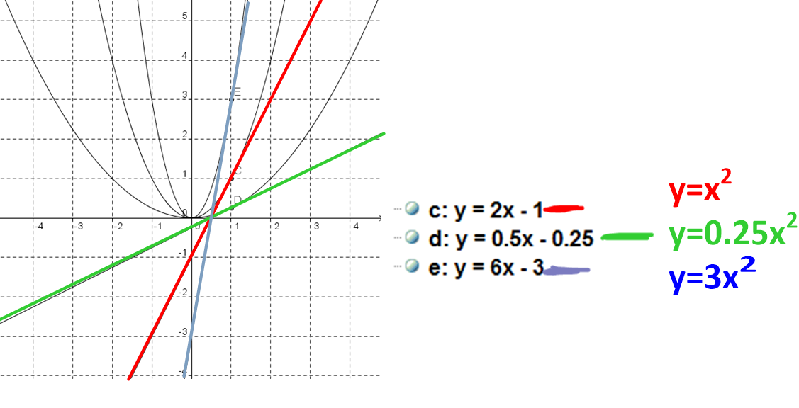
. , then we know that the slope of the transformed function is
  .
. .
. is, they immediately think (or at least can understand) that we get
  , because…
 which has derivative (aka slope of the tangent line)
  … Thus the transformed function
  is going to be a vertical stretch, so all the tangent lines are going to be stretched vertically by a factor of 9 too… thus the derivative of this (aka the slope of the tangent line) is
  actually means. Why does it need to be there to calculate the instantaneous rate of change. (Be sure to address with h means.)
 gets closer and closer to -1. Thus if we bring h infinitely close to 0, we see that
  at
at 
