Multivariable Calculus

MV Calculus Projects 2010-2011

One class that I think I am pretty free about, and we have some fun in and get to explore and go through a lot of productive frustration, is my multivariable calculus class. I had 5 students in it last year. (*As he ducks from the rotten vegetables hurled his way, and collective groan from the crowd.*) Sadly, next year, there will be no students eligible so I won’t be teaching it.

My favorite thing from this course is the fourth quarter projects that all students do. We don’t have problem sets, we don’t have any tests or quizzes. Just this thing.

At the beginning of the year, I tell students to write down random things that pique their interests, whet their appetites, for the fourth quarter project. Whether it be higher dimensions, to the notion of curvature and what that might mean for surfaces, to the use of optimization problems in various fields, to whatever. As the class goes on, I’ll mention some interesting tidbit here or there and sometimes they’ll add it to the list in the back of their notebook. And then comes the fourth quarter, where they basically get to pick anything they want, they write their own project prospectus, they write their own rubric, and they just go at it. I give them some options, but they don’t always go that way.

I meet with them once a week or every other week (or more if they need it) and provide guidance and support, sometimes needed, sometimes not.

This year I had some excellent projects. I can’t believe I didn’t outline them for you when we finished the year, so I will outline them now. What was great is that some parents got to come to the final presentations, and so did my department head, the head up of the upper school, and some math teachers. Different days had different audiences.

1. The first project involved constructing 5 intersecting tetrahedra out of origami and figuring out the “optimal strut width” (the width of the “beam” of each edge of the tetrahedra) so the tetrahedra just sit beautifully within each other without having them wiggle around (too small) or bend to fit together (too large).

This problem involves multivariable calculus, believe it or not, but also involved some really beautiful precalculus work meshed with 3D (basically, using roots of unity and some right triangle trigonometry) to find the vertices of a dodecahedron. I also have to say that making the darn thing was totally hellish and the student who did it is a super rockstar. She also wrote a really comprehensive final paper explaining the calculations. Color me impressed.

2. Another student, who is a nationally recognized runner, wanted to investigate the following question: if you have a random surface with a local maximum, and you put yourself on that surface, and you wanted to get to the maximum, how would you get there? Instead of taking the shortest path (which would follow the gradient), the student conjectured that if you ran along the least steep path you will run faster, and if you run along the most steep path you will run slower. So there is a tradeoff, and there will be a path to run in between those two choices which will be optimal. So the student and I constructed a function to model the velocity of this runner. Although together we couldn’t actually get a general answer, or even a specific answer for a specific surface and point we chose, we had fun struggling through it. The student also created an accurate model of a one surface that the runner would be running on (the one that he did his calculations for).

3. Another student, for an earlier problem set where they were asked to write their own problems, studied the idea of marginal utility in economics and related that to Lagrange multipliers. This student was one of those kids who is interested in everything and he really loved studying marginal utility, and wanted to extend it and see how else multivariable calculus was used in economics. So he pretty much devoured this book on his own. Although he didn’t find too much multivariable calculus, he became enamored with the idea of the utility function, and decided to make a 50 minute class lesson on economics and calculus with an emphasis on the utility function. It was so well thought out, and so well delivered, that I think that teaching and simplifying ideas might be this kid’s calling. He also wrote an amazing paper outlining everything from the presentation (and more that he couldn’t fit in), and a problem set for students to work on after the presentation.

4. Say you have a blob drawn on graph paper, and you wanted to measure the area. What if I said: there is a mechanical device that if you drag it along the perimeter of the blob, it would calculate and tell you the area? True story, this exists, and when I described this to a student struggling to find a project… a project he was insistent he wanted to make with his hands… he was hooked. The device is called a planimeter. It sort of makes sense that something like this could exist… I mean:

(that’s Green’s theorem). So this mechanically minded student first built a trial version of a planimeter, using pencils, binder clips, and a bottle cap. And it worked fairly well. So then he built a giant and much more sturdy one. You can see this student holding his “draft” version and on the table is his professional version.

This student did almost all the work without me (which is good because I have no idea how to work with things mechanically). I basically only helped him understand some of the math behind how the mechanical device worked. The end result was that the professional device worked fairly well, but I think given another week, it could have been tenfold more accurate. Time is always the sticking point with these end of year presentations.

5. The final project was one of my favorites, because it involved me really going back and learning some simple partial differential equations. How this project happened involved me showing this student the following video:

Of course this video can’t but help stir the imagination. So this student wanted to build the device (called a Chaldni plate) and study the math behind it. It turned out that building the device was a bit beyond our capabilities, so we enlisted the help of the science department chair who super generously ordered a chaldni plate (he had the driver already) and helped get him set that up. I, on the other hand, did some research on what causes those beautiful patterns. Together, that student and I spent hours upon hours tearing through a paper — me doing a little lecture, him reading and asking questions, and so on and so on. And at the end, this student wrote his own paper based on our reading — explaining the math behind the designs. Although I don’t think he fully understood everything (we had not nearly enough time to make that possible), I loved that he got a touch of all these small things in higher level math. Orthogonal functions and Fourier series. 2D and 3D waves. Boundary conditions and time-dependent partial differential questions.

And his Chaldni plate worked.

PS. Apparently, I didn’t do a good job of blogging about my projects from previous years. Two years ago, here is what my kids did. And last year, I didn’t really write about it. Yikes! One student did a wonderful investigation on higher spatial dimensions, and how to extend what we’ve done into them — focusing on actually visualizing these dimensions (she really really really wanted to see them). The other extended a 2D project on center of mass that someone worked on the previous year, and I wrote about it obliquely here.

Nothing here nor there

This is a post with things neither here nor there. Mainly because I’m too tired to come up with something focused and comprehensive.

1. I’ve been cribbing a lot from Kate Nowak for my logarithm’s unit in Algebra II this year. I used her Log War cards again, to great success, and I cribbed one of her smartboards and converted it to a partner worksheet for kids to discover the log laws. So three cheers for Kate Nowak! I also had students read aloud @cheesemonkeySF’s translation of Napier’s introduction in class. So three cheers for @cheesemonkeySF and Napier!

2. I am feeling anxious about my senior letter this year. What am I going to say? I’ve started and deleted it twice.

3. I have had (and continue to have) a lot of social events on my calendar. This is not good considering all the work I have to get done.

4. I’m getting a little anxious about my multivariable calculus projects. I have 5 students to keep track of, and I don’t have a good sense of where a few of them are. I just sent out an email to the rest of the math department inviting them to join us for the project presentations/project share.

The Multivariable Calculus Class would like to formally invite you to hear about the work we’ve done this last quarter on our final projects. The students in this class have independently worked on:

1. Stu 1: Explaining foundational college level economics with a focus on utility functions
2. Stu 2: Building a model of a 3D hill-like function and using that model to teach some fundamental multivariable calculus topics
3. Stu 3: Building a beautiful origami sculpture (5 intersecting tetrahedra) and using multivariable calculus to figure out the optimal size of paper to use so the sculpture perfectly interlocks
4. Stu 4: Building a machine that can measure the area of any irregular (and regular!) figure — because it is enacting Green’s Theorem
5. Stu 5: Building a special instrument which does something special with sound (I am not saying more for the element of surprise) — an investigation which delves into physics, partial differential equations, and fourier series.

If you are free, we would love to have you join us as we share the projects we’ve worked on with each other.

Stu 1’s project will be presented on Monday, May 16th at the start of B band (9:30-10:20)
Stu 2’s and Stu 3’s projects will be presented on Wednesday, May 18th at the start of B band (8:35-9:25)
Stu 4’s and Stu 5’s projects will be presented on Friday, May 20th at the start of B band (8:10-9:00).

We are in the room S201.

Always our best,
Stu 1, Stu 2, Stu 3, Stu 4, Stu 5, Mr. Shah
The Multivariable Calculus Class

5. I am doing this summer program called the Klingenstein Summer Institute. Part of what we were asked to do is to videotape one of our classes. I did it, and I’m not going to watch it (they say not to). Right afterwards, I actually thought it went fairly well… although my timing was off, I felt the class was solid. Of course, we were asked to reflect upon the class. And the more I thought and parsed and analyzed, the more I came to the realization: the class wasn’t actually very good. It wasn’t bad, but it wasn’t very good.

They also asked me to email a headshot for a facebook they are compiling. I attached this gem from years ago.

That’s because in most of my photos, I look like:

so my selection is limited.

6. I am getting more and more excited about the second summer program I’m doing called the Park City Math Institute. I did it last year, and it was fantastic, times a million. I can’t recommend it highly enough.

7. I was told today that some kids in a senior homeroom were randomly singing my praises. Which made me melt a little. Okay, a lot.

8. I’ve been listening to this GLEE song on the way to school to wake up and get psyched for the day. I haven’t been sleeping a lot, so this is needed.

9. Today I went to a used book store that was going out of business and bought Volume 1 and Volume 2 of Polya’s Mathematics and Plausible Reasoning. Hardcover. Pristine condition. First printing. Beautiful. (I also bought a copy of Jude the Obscure and Surely You’re Joking, Mr. Feynman. I think I own both, but I love both. And they were only a few bucks.)

Books! Books! Books!

I’ve been a bit incommunicado lately. Nothing bad has happened! I’m not working harder than normal! I don’t know why but I haven’t been moved to post anything. And you know my feeling about blogging — it can’t be a chore, so don’t force it.

That being said, I wanted to share something we’ve been diverted by in multivariable calculus recently:

I gotta say, I love this class and I love working with these kids. They remind me how when you find the right thing, exploration is captivating.

This is the “book overhang problem.” The question we dealt with was: can you stack books at the edge of a table so that the top book is off the table completely (meaning if you’re looking down on the stack of the books, the top book doesn’t lie over the table at all)?

We haven’t yet found the optimal solution, but we’re going to be discussing our musings on Friday — what the best 3, 4, and 5 book configuration might be, and if we can generalize it.

fnInt reprise

My last post was about how the TI-83/84 calculates integrals (how fnInt works), and how it messes up for when you have large intervals.

I just came from my Multivariable Calculus class, where each student had done some thinking about it. One investigated the Gauss-Kronrod quadrature. A couple others played around with fnInt and came up with some bounds for when fnInt was good and when fnInt was bad for our function $f(x)=e^{-x^2}$ .

What we did today was to start investigating fnInt in a different way. (Yeah, my goal was to start triple integrals today… but this was way more exciting in the moment…)

We looked at $\int_1^{\infty} \frac{1}{x^2}dx$ and used fnInt to calculate it.

It turns out that fnInt goes crazy and fails to be a good estimator at a particular large interval.

So we continued looking at $\frac{1}{x^3}$ , $\frac{1}{x^4}$ , $\frac{1}{x^5}$ , etc. We looked at where fnInt broke down.

This is what we found out:

The left column is the exponent in $\frac{1}{x^n}$ . The right column is the last integer you can integrate (using fnInt) to so that doesn’t give a terrible estimation of the area. (Recall we’re integrating from 1 onwards, not from 0.)

My kids are going to go home and see what they can make of this data. We hope we can use it to come up with a prediction for where fnInt will go awry for estimating the area for something like $\frac{1}{x^{43}}$ ? And maybe it’ll also work for non-integral values, like $\frac{1}{x^{3.23}}$ ? We’ll see.

…Hopefully we’ll start on triple integrals soon, though…

TI-83/84 Question

Today in multivariable calculus, we were talking generally about $\int_{-\infty}^{\infty} e^{-x^2} dx$ . Before we embark on evaluating this integral, I wanted kids to guesstimate using their calculators what the value is.

The calculator image showed:

They had a conjecture as to what was going wrong when we expanded the interval… the calculator might be doing a finite number of Riemann Sums, then the width of each rectangle would be large andthe height (especially near the hump near 0) would be small.

Okay I’m describing it terribly… maybe a terrible picture will help.

Good conjecture. Great conjecture, in fact. But I doubted that the TI-83/84 uses Riemann Sums to do fnInt.

It was the end of class, so I sent my kids off with this one charge: investigate how the TI-83/84 calculates integrals, and see if you can’t explain why we’re getting funky answers for a large interval.

I figured I’d pose the question to you, if any of you are calculator saavy…

I wonder if it has to do with the fact that the calculator can only store so many (is it 15?) digits — as part of it?

PS. My very limited research has led me to the fact that the calculator does something called Gauss-Kronrod quadrature, which is a lot of gobbly gook to me right now.

Multiple Integrals! Jigga Wha?!

In Multivariable Calculus today, I let my kids loose. We are starting our chapter on multiple integrals, and I generally start out just dryly explaining what integration in higher dimensions might look like. But today, I decided to scrap that and have my kids try to see if they could generalize things themselves and come up with an idea of what integration in multivariable calculus would look like.

It was awesome. They immediately picked up on the fact that it would give you (signed) volume. That was great. They realized the xy-plane was equivalent to the x-axis. With some prompting, they understood we weren’t integrating over a 1D line (like between x=2 and x=5 on the x-axis), but now on a 2D region. (Of course, a little later, I explained that they could integrate over a line, but they’d get an area.)

Here’s the final list we generated.

It was nice, because students were coming up with some pretty complicated ideas on their own. They were motivating things we were going to be learning. Nice.

After we went through this thought exercise, still not looking at a single equation, I then threw the following up on the board:

I wanted to see if they could use our discussion to suss out some information about the notation, and the meaning behind it. They actually got that the limits 2/4 correspond with y and the 0/3 correspond with the x. And that the region we’re integrating over is a rectangle. And the surface we’re using is $4-2xy$ . I mean, they got it.

I then showed them how to evaluate this double integral, briefly. I tried to get the why this works across to them, but we ran out of time and I slightly confused myself and got my explanation garbled. I promised that by the next class, I would fix things so they would totally get it.

Although not perfect (but good enough for me, for now), I whipped up this worksheet which I think attempts to make clear what is going on mathematically.

View this document on Scribd

I strongly believe, however, that this will drive home the concept way better than I ever have done before. If you teach double integrals, this might come in handy.

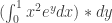
PS. I, a la Silvanus P. Thompson in Calculus Made Easy, talk about dx and dy as “a little bit of x” and “a little bit of y.” So if you’re wondering what I’m looking for question 2 on p.2, I want students to say dy. Then the answer to A is $(\int_{0}^{1} x^2 e^y dx)*dy$ . That’s the volume of one infinitely thin slice. Now for B, we have to add an infinity of these slices up, all the way from y=0 to y=2. Well, we know an integral sign is simply a fancy sign for summation, we so just have $\int_{0}^{2} (\int_{0}^{1} x^2 e^y dx)dy$

3D Maxima and Minima

In multivariable calculus, we were finding relative maxima and minima. It’s much like finding maxima and minima in 2D.

The general idea in 2D is that if you go a little bit to the left or a little bit to the right (changing x by a wee bit) at a maxima or minima, you aren’t really changing your height much (you aren’t changing y by much). Another way to look at it… if you zoom in enough to a maxima or minima, you’ll almost see a straight line! And you can make it as “straight” as you want it by zooming in more and more and more.

Does that make sense?

Now we do a similar argument for maxima and minima in 3D:

At the top of peaks or troughs, you’ll notice if you walk a wee little bit in the x direction, the height (z) isn’t changing by much. Similarly if you move a wee little bit in the y direction, the height isn’t changing as much. (Or, analogously, if you zoom in a lot lot lot lot, you’ll be looking at something almost perfectly flat, a horizontal plane…)

In other words, instead of saying maxima and minima only occur when $f'(x)=0$ , we now can say that maxima and minima only occur when $f_x(x,y)=0$ and $f_y(x,y)=0$ . That’s the mathematical way to talk about moving a bit in a x-direction or y-direction.

So my kids know to find possible relative maxima or minima, you have to find the points $(x,y)$ which make $f_x(x,y)=0$ and $f_y(x,y)=0$ .

In class I then posed a few good questions:

(a) If you know a maximum occurs at the point $(2,3)$ , how can you show that the directional derivative in the direction $<\frac{1}{\sqrt{2}},-\frac{1}{\sqrt{2}}>$ is also 0?

(b) If you know that at the point $(5,7)$ , the directional derivative for $<\frac{3}{5},\frac{4}{5}>$ is 0, and the directional derivative for $<\frac{1}{\sqrt{2}},-\frac{1}{\sqrt{2}}>$ is also 0. Prove that the point $(5,7)$ is a maximum or minimum or saddle point.

These were things that I thought up on the fly… it’s interesting. We get so used to procedures, that we sometimes forget what they mean. The point I was trying to make is that if any two (different) directional derivatives were 0 at a point, then that point could be a maxima or minima. If you pose that as a claim, and students are used to thinking algebraically, they have to go through the motions to see this is true. (It basically involves creating and solving a system of two linear equations…). [1]

But there’s a much easier way to get students to buy that claim. If you think graphically, this makes sense… if you are at a maxima or minima, and you zoom in enough, the surface will look like a flat plane. So of course if you walk a short distance in any direction, you shouldn’t be moving (much) in the $z$ direction.

I don’t know… this isn’t deep or anything. But it was something that I didn’t plan in class that I thought was interesting…

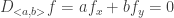
[1] This is how it would go… Assume you know $D_{<a,b>}f=0$ and $D_{<c,d>}f=0$ (and the two vectors aren’t scalar multiples of each other). Then you can rewrite $D_{<a,b>}f=af_x+bf_y=0$ and $D_{<c,d>}f=cf_x+df_y=0$ . Well then you simply have a system of equations that you can solve for $f_x$ and $f_y$ — and it is easy enough to show that the solution is $f_x=0$ and $f_y=0$ .