Multivariable Calculus

Arc Length of Lissajous Curves, or Pretty, Pretty Pictures!

In MV Calc today, we were learning about arc length. In 3D, if you have parametric equations defining a curve, you can find the arc length by calculating:

L=\int_a^b \sqrt{(\frac{dx}{dt})^2+(\frac{dy}{dt})^2+(\frac{dz}{dt})^2}dt

I asked them to calculate the length of this curve, which will repeat itself, over and over and over:

x(t)=\cos(3t), y(t)=\sin(5t), z(t)=\cos(2t)

If you graph it, it looks like this (it’s a 3D Lissajous curve):

Vodpod videos no longer available.
more about “2008-10-27_1849“, posted with vodpod

Which is awesome! They had to figure out the limits of integration (the function will go back to it’s original starting point when t=2\pi, so the limits of integration are from 0 to 2\pi. And we had to use our fnInt function on our graphing calculators to actually calculate the length. But it was cool.

During the class, I starting thinking of all the extensions and projects that could come out of this. For example, we could have students study x(t)=\cos(at), y(t)=\sin(bt), z(t)=\cos(ct). If a, b, and c are all rational numbers, we can prove that the curve will repeat itself. However, as soon as we make one of them irrational, we can prove the curve will not repeat itself. Look at this video to see how cool it looks!

Vodpod videos no longer available.
more about “2008-10-27_1852“, posted with vodpod

What if all three (a, b, and c) are irrational? What constraints do we need if we want the function to repeat? (The answer won’t be tough, I imagine, but worth exploring.)

Also, on the subway ride home, I wondered if we could come up with an explicit formula (rather than parametric) for a surface containing every point on the curve. (A harder question, for sure.)

And another: what is the smallest volume you can design to enclose a curve which does repeat, like x(t)=\cos(3t), y(t)=\sin(5t), z(t)=\cos(2t). Since sine and cosine bounce between 1 and -1, I will say that your volume had better be better than 2^3.

Terminology, Notation, Ideas

In my (non-AP) calculus class last week, I was teaching my students about continuity of a function. Before we started, I asked them what continuity was, and students in both sections started their answer by saying “well, it’s when you draw a function and you don’t have to lift your pencil.” Some spoke of holes and asymptotes. Others spoke of endpoints.

I then proceeded to wow them by saying — all that they said could be encapsulated mathematically. The act of tracing out a function knowing where you’re going to have to lift it can be rewritten with three rules. They weren’t as impressed with that fact as I was, but I still tried to convey “Think about it! You can translate moving your hand across a page smoothly into mathematical statements.”

What’s needed for continuity of a function f(x) at x=c:

1. f(c) is defined
2. \lim_{x \to c}f(x) exists
3. \lim_{x \to c}f(x)=f(c)

I did the most obvious *you need to memorize this for tomorrow* wink-wink nudge-nudge that I possibly could. I might have even *coughed* the words “pop quiz.”

I just graded the quizzes. Horrible. HORRIBLE.

I got things that show no understanding of the symbols of calculus or what continuity means. Some examples:

(a) function f(x) exists
(b) f(x)=f(c)
(c) \lim_{x \to c}f(c) exists
(d) one value for f(x)
(e) the two-sided limit of c exists
(f) the two-sided limit of x is equal to c
(g) the function has to be continuous (you cannot pick up the pencil)
(h) \lim_{x \to c}f(x)=c

There are some major notational misunderstandings, but also part and parcel, some conceptual misunderstandings. I mean, for example, “the two-sided limit of c exists” doesn’t really mean anything useful to us. First of all, it should be the limit of the function, and second of all, it doesn’t say the limit as x approaches something.

I typed a bunch of these out and we’re going to talk about them in class tomorrow. Hopefully we’ll get to parlay that into a discussion of notation, the precise meaning of math symbols, and the importance of listening to Mr. Shah’s coughs.

Multivariable Calculus Problem Sets

As you probably know, I’m teaching Multivariable Calculus this year, and I came into the course with a vision: a collaborative, problem-solved based class, where students aren’t motivated by exams and grades, but rather by the challenge of thinking for themselves.

(Of course, getting really great, full-of-personality students helps too!)

The problem sets seem to be working out well. (As of now, I’ve gotten or adapted most of the questions from Anton; but I’m going to be integrating more questions from other sources.) At the end of the course, I’ll probably post them all my Multivariable Calculus Website, but for now I’ll post what they’ve been given:

multivariable-calculus-problem-grading-rubric
problem_set_1a
problem_set_1b
problem_set_2a

Of course I’ll be asking my students to reflect about this course, and the problem sets, and the very different setup. I’m more than curious as to what they’re going to say. I’m also hoping to get permission from my students to scan in their solutions, so you can see the evolution (or not) of how my students communicate mathematics.

You can see two of my favorite problem set problems below.

A Great Moment With Spherical Coordinates

In my multivariable calculus class yesterday, I was introducing spherical and cylindrical coordinates. These students didn’t take precalculus, so they didn’t have a ton of practice with polar coordinates. So I thought it was going to be a tough class to teach. To compound that, the smartboard wasn’t working, so I couldn’t show them some great demonstrations (here and here).

We had to do things by hand.

And I wanted to spend the entire period working on deriving the conversions:

Given a point in rectangular coordinates, how do you find the cylindrical coordinates?
Given a point in cylindrical coordinates, how do you find the rectangular coordinates?
Given a point in rectangular coordinates, how do you find the spherical coordinates?
Given a point in spherical coordinates, how do you find the rectangular coordinates?

And we went through it all. It wasn’t easy, but they “saw” it. They came up with the conversions. I just guided them.

I had two favorite moments in this class:

(1) At one point, when dealing with spherical coordinates, one student discovered an equation for the angle made with the positive z-axis. The equation wasn’t the one in the book. I suspected the two were the same, but decided I wasn’t going to pursue it. A student said we couldn’t leave it hanging, we HAD to figure it out. So we did, together. That 7 minute aside was awesome.

(2) The school clocked stopped at one point, and of course, it was noticed by a student. (Do my students wait with hungry eyes for the course to end?) Apparently the clocks in the school do that occasionally. And somehow, in a fit of impulsivity, I got onto an aside about standardizing time, Einstein’s work in the Patent Office in Switzerland, and his original 1905 paper on special relativity. (See Peter Galison’s Einstein’s Clocks, Poincare’s Maps if you want a lengthy version of what I told them.)

Cross Products

So I was teaching the cross product in my multivariable calc class on Friday. For those who are a bit rusty, \vec{a} \times \vec{b} is the notation for the cross product between 3-dimensional vectors \vec{a} and \vec{b}. It is defined as:

Prompted by a question from a student, I was struck with two related questions. One is: why does \vec{a} \times \vec{b} yield a vector orthogonal to both \vec{a} and \vec{b}? That question doesn’t mean I want a proof: I can do that. But I want some intuitive sense of why it works.

The second question is: can we find cross products in other coordinate systems, in the same way? How generalizable is this whole “take the determinant of a 3×3 matrix”? Would finding a cross product using a determinant work in, say, spherical or cylindrical coordinate — where instead of putting \vec{i}\vec{j}\vec{k} as the top row of the matrix, you put the fundamental unit “direction” vectors in these other coordinate systems? I haven’t played around with these coordinate systems in a long time, but I suspect the answer is no. (And to see that, I’d just have to do a simple test case, which wouldn’t work out… and that ought to be good enough.) I have to run to a picnic now, so maybe I’ll try this out later.

Hm, this looks like it could be turned into a good question for the next problem set, or even a good project for the multivariable students.

This train of thought also got me musing on the “what are the origins of vector analysis?” question. I haven’t had time to do any serious research, but it appears that one important book on this question is A History of Vector Analysis by Michael Crowe.

Course Expectations for an Unusual Course

So next year — as you might know from various posts this summer — I’m teaching Multivariable Calculus. I’ve spent this summer trying to refresh myself with the subject, which has remained dormant in a portion of my brain which has been unused since 1999.

The thing that has been weighing on me is how different this course is, in terms of both content and in terms of the class makeup itself. Here are the things I was grappling with when designing the course:

  1. The course will have only 2-4 students in it.
  2. The students are going to be pretty advanced who have shown they can do high school level math, and well. [1]
What I want students to get out of the course:
  1. The obvious and the most crucial: I want the students to understand the basics of MV Calculus
  2. I want students to acquire and master problem solving skills. By the end of the course, I want students to see that math problems can require more than 1-3 minutes each, and there are wrong directions that need to be taken.
  3. I want students to learn that math can be a collaborative activity. I want to foster a class atmosphere where we all are working together to conquer the material.
  4. I want students to learn to communicate math effectively — both in written form (in terms of writing the solutions to problems) and in verbal form (in terms of explaining concepts).
  5. I want students to become familiar with the use of computer software to help solve problems which don’t have algebraic solutions (or involve a lot of manipulation).
With these goals in mind, I designed the course. [I think I dealt with all but #5, which is because I haven’t yet learned how to use SAGE Notebook (here). But when I do, I will incorporate questions and tutorials in the problem sets.]
But I’m nervous. It’s so different that I wanted to solicit any feedback. So if you have the time (and desire), take a peek below at the course expectations and tell me if there is anything that looks like it won’t work. (Or if there is something that looks like it will work well.)
(download pdf here or by clicking picture above)


I initially had designed this course with no tests, but I added in a few out of the fear that students — especially seniors who are going to be bombarded with work from other classes — would easily turn this course into a “back burner” course. Meaning that they would go home with a lot of homework and decide that the one course they could sacrifice (or do halfheartedly) would be math, because there was so little accountability.
And if you’re curious what the problem sets might look like, I am copying two questions (both cribbed from Anton) below.
[1] I haven’t taught any high school honors/advanced courses yet, so this is new territory for me.

Polar form of Laplace’s Equation

As you might know, this summer I’m prepping for the multivariable calculus course I’m teaching next year. When going through the textbook, I’m attempting some of the “challenging” problems near the end of the section.

Today, when refreshing myself with the chain rule, I came across a problem which tested my intuition. And I’m afraid I’ve lost what little intuitive mojo I had years ago. I’m going to reproduce the problem below.

Question:

Suppose that the equation z=f(x,y) 
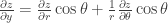
is expressed in the polar form z=g(r,\theta) by making the substitution x=r \cos \theta and y=r\sin \theta.

  1. View r and \theta as functions of x and y and use implicit differentiation to show that:
    \frac{\partial r}{\partial x}=\cos\theta
    \frac{\partial \theta}{\partial x}=-\frac{\sin\theta}{r}
  2. View r and \theta as functions of x and y and use implicit differentiation to show that:
    \frac{\partial r}{\partial y}=\sin\theta
    \frac{\partial \theta}{\partial y}=\frac{\cos\theta}{r}
  3. Use the results in parts (1) and (2) to show that:
    \frac{\partial z}{\partial x}=\frac{\partial z}{\partial r}\cos \theta-\frac{1}{r}\frac{\partial z}{\partial \theta}\sin\theta
    \frac{\partial z}{\partial y}=\frac{\partial z}{\partial r}\cos \theta+\frac{1}{r}\frac{\partial z}{\partial \theta}\cos\theta
  4. Use the results in part (3) to show that:
    (\frac{\partial z}{\partial x})^2+(\frac{\partial z}{\partial y})^2=(\frac{\partial z}{\partial r})^2+\frac{1}{r^2}(\frac{\partial z}{\partial \theta})^2
  5.  Use the result in part (4) to show that if z=f(x,y) satisfies Laplace’s equation
    \frac{\partial^2 z}{\partial x^2}+\frac{\partial^2 z}{\partial y^2}=0
    then  z=g(r,\theta) satisfies the equation
    \frac{\partial^2 z}{\partial r^2}+\frac{1}{r^2}\frac{\partial^2 z}{\partial \theta^2}+\frac{1}{r}\frac{\partial z}{\partial r}=0
    and conversley. The latter equation is called the polar form of Laplace’s equation.
Here’s my issue. I can do parts (3)-(5) fine. But I got stumped for a good 15 minutes on the parts (1) and (2) and I’m sad about it.
So my lament is: wow, I suck.
And my question is: is there an easier way to solve this?
My solution is the following:
We know y=r\sin\theta, so differentiating with respect to x we get
(1) 0=\frac{\partial r}{\partial x}\sin\theta+\frac{\partial \theta}{\partial x}r\cos\theta
We know x=r\cos\theta
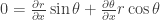
, so differentiation with respect to x we get
(2) 1=\frac{\partial r}{\partial x}\cos \theta-\frac{\partial \theta}{\partial x}r\sin\theta
We now have a system of two equations, which we can solve for \frac{\partial r}{\partial x} and \frac{\partial \theta}{\partial x}. Going through the motion yields the right answer.
So yeah, looking back, its all makes sense. And I feel sheepish for posting this, because this is pretty easy to do. But it doesn’t seem simple. There is a part which calls for intuition: to know that we have to get two equations and then solve them together. I’m guessing there’s an easier way to do this, that doesn’t involve solving a system of equations. Is there?