Month: January 2009

Completing the Square

Yesterday I ahem-ed and winked to my Algebra II class about them needing to know how to complete the square for class today. Teaching this topic last year was a nightmare. A total trainwreck. Students were having difficulty all over the place — they couldn’t simplify radicals, they didn’t get why the procedure worked, they were wondering how imaginary numbers came into play here, they confused the steps, they didn’t *get* it. And it was my fault.

Part of the problem was that we were doing too much, too fast. We had brought in graphing quadratics early on, and we were emphasizing the relationship between the equations and the graphs from the start. We also — in the middle of the quadratic unit — taught complex numbers. That’s too many huge things to deal with. Quadratics bring too much together, and we needed to keep the ideas and skills organized so they make sense.

So the other Algebra II teacher and I decided we’d try something different. First, this year, we introduced complex numbers without talking about quadratics. We motivated these numbers, and then we had students practice working with them, getting really comfortable with them. Second, when we started quadratics, we did so without any graphing. Period. We were doing all algebraic work.

Here’s how we progressed.

PART I: Review
Regular, very simple equations with solutions involving square roots, imaginary numbers, and real numbers:

quad1
Quick review of factoring:

quad2

A brief discussion of solving equations with perfect square terms — with imaginary and real solutions:

quad3

Part II: Completing the Square

Perfect Squares:
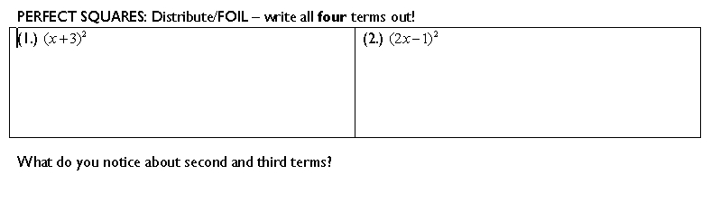
quad4

We talked about what a perfect square is and noticed a relationship between the four terms — when you FOIL. Importantly, students are going to see that the second and third terms are the same.

***

Creating Perfect Squares!:

quad5

The next step of creating perfect squares really has them grapple with the fact that the missing constant term is simply half of the coefficient of the x term squared.

***

Completing the Square:

quad6

For me, it was this step, just a short distance from the last step, which made the entire unit a success. Because now my students had seen the relationship between all the terms in a perfect square and actually seemed to understand them. My favorite part was that most students were getting problem 10 right — and it involves fractions! We also talked about how important signs are for this process.

***

The End Game: Completing the Square

Before we actually “completed the square” I had students look at the last section of the review sheet.

quad3

We talked about how if you can write a problem in this form, that you can ALWAYS solve it. And what we were going to be doing is finding a way to write any quadratic equation in that form, so we can solve it.

Then, I went through an example — step by step — to get a problem to that form:

quad7

Then I had them solve it, like they had done previously. Most of them had no trouble solving it.

quad8

They practiced doing a few problems on their own — some which gave “nice” answers, some which gave answers with radicals, and some which gave complex answers.

Part III: Reinforcement

I made them practice a few more times, with some harder problems, and then I threw them a curve ball — a coefficient in front of the x^2 term. We conquered that, although there were same difficulties with fractions. Then I put some terms on one side and some terms on the other side (e.g. x^2=2x-15).

Overall, they really rocked it. How do I know they got it?

I started off this post by saying that I ahem-ed about giving a pop quiz in my class today. Well, I followed through on that. gave a pop quiz to my class on completing the square. I gave them one easy problem and one much more difficult problem — with fractions and radicals — on completing the square.

I got a whole bunch of perfect scores.

If you want, the worksheets I created are below:

Factoring Quadratics
Completing the Square, Part I
Completing the Square, Part II
Completing the Square, Pop Quiz

L’Hopital

Today a student in my calculus class asked why L’Hopital’s Rule works. I paused, and failed to think of an easy way to explain it. But now I’ve found a really easy way to explain it — at least for the 0/0 case. (Thanks Rogawski!)

We want to show that \lim_{x\rightarrow a} \frac{f(x)}{g(x)}=\frac{\lim_{x\rightarrow a} f'(x)}{\lim_{x\rightarrow a} g'(x)}.

At least in the 0/0 case, we know that f(a)=0 and g(a)=0. Great! If that be true, we can say that:

\frac{f(x)}{g(x)}=\frac{f(x)-f(a)}{g(x)-g(a)}

Of course that has to be true, because we’re subtracting 0 from the top and the bottom! Now we can say:

\frac{f(x)}{g(x)}=\frac{\frac{f(x)-f(a)}{x-a}}{\frac{g(x)-g(a)}{x-a}}

(We are dividing the top and bottom by the same number.)

Finally, we take the limit as x approaches a of both sides, to get:

\lim_{x\rightarrow a}\frac{f(x)}{g(x)}=\lim_{x\rightarrow a}\frac{\frac{f(x)-f(a)}{x-a}}{\frac{g(x)-g(a)}{x-a}}

By basic limit rules, we can rewrite the right hand side of the equation to be the limit of the top and bottom separately. But the limit of the top and bottom separately are just the derivatives! (See the definition of the derivative there?)

\lim_{x\rightarrow a} \frac{f(x)}{g(x)}=\frac{\lim_{x\rightarrow a} f'(x)}{\lim_{x\rightarrow a} g'(x)}

Q.E.D.

This Sunday: A Meandering Post

Today was exhausting. It’s been a while since I really, really planned for classes. The past week was this weird interim week where I didn’t work full-force. Midterms were canceled and classes continued, but in this half-hearted way. So it’s been a bit of a shock to sit down and plan 3 lessons, and do a giant pile of grading.

I counted. Today I graded 216 papers, which consisted of 600 problems (not counting parts a, b, and c as separate problems). I created 57 SmartBoard slides (well, some I cribbed from last year, or from previous classes). I entered 24 grades in my gradebook. I modified and printed one worksheet on the quadratic formula. I created my next problem set for my Multivariable Calculus class [1]. I set up my calendar for the next two weeks. Go me!

The next week is going to be brutal — the start of a new quarter, along with the task of entering and finalizing all the grades from the previous quarter.

I’m actually nervous about this upcoming week — but not only because of the work I’m going to have to do. Because of the student death at my school, two weeks ago, everything has been in disarray. Midterms were canceled, tests were modified to be open note or take home, movies were shown in classes (including some of mine), and students were given lots of flexibility. (“You were unable to focus last night? Of course you can take the quiz in study hall tomorrow.”) In other words, for the past two weeks, I unclenched my fist. My expectations were blurred. They were also greatly lowered. Starting tomorrow, I have to go through the process of re-clenching my fist. It’s going to be hard. I’m going to be clear with everyone that even though we’re not going to be the same, life has to go on in my classes. We’re going to go full force, and I am going to have the same high expectations for everyone that I had earlier in the year.

Here’s to hoping that the transition will go easily. I believe that as long as I’m clear with them, they’ll rise to the occasion. They have in the past.

[1] Actually, this problem set is going to be different from the others, and I’m hoping pretty interesting. I am assigning them one problem on using multivariable calculus to find the line of best fit (some of them are concurrently taking statistics), and then they are asked to create their own problem set for the material we’ve covered. Three problems. One which they have to make up themselves, but they can be inspired from any resources. The other two can come from other resources. Heck, you can read the problem set here. I’m hoping that having them dig for problems that seem interesting to them will keep them excited about the material. I’ll let you know how that goes.

In fact, here are all my problem sets so far.

multivariable-calculus-problem-grading-rubric
problem_set_1a
problem_set_1b
problem_set_2a
problem_set_2b
problem_set_3a
problem_set_3b

dy/dan’s “Feltron” contest

Just a quick link passing you along to Dan Meyer’s Annual Report contest.

Design information in four ways to represent 2008 as you experienced it. This can mean:

  • four separate PowerPoint slides with one design apiece,
  • one JPEG with four designs gridded onto it,
  • an Excel spreadsheet inset with four charts,
  • etc.

I had a blast working on it last year. To get a sense of what we’re talking about, check out examples from last year.

Day Six: The Memorial Service

The memorial service for the student who passed away last weekend was held today. I went with a group of teachers so we could support each other and students. The church was packed and hushed, and the service was emotional. Students — his friends — spoke about their memories of the deceased, and about his best qualities, and about the love that exists between friends. The pain in the tremors in their words was hard to hear. That was the hardest part of being there for me. But hearing all the wonderful memories, how much this person touched those around him with his large heart and humor-filled personality, was also the best part about being there too. I almost cried when someone read “Goodnight Moon,” which was one of his favorite books when he was a child.

A few of us went out for a late lunch afterwards and just being around each other was helpful. Not that I’ll ever forget this incident, and surely there is still going to be an aftermath for weeks to come, but with this, I think I’m done talking about it on this blog. There’s probably just going to be one more post about how this relates to teaching at some point in the future.

Goodnight stars
Goodnight air
Goodnight noises everywhere

Why is the gradient related to the normal vector to a surface?

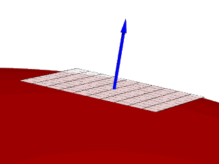
Today in Multivariable Calculus I was supposed to teach my students how to find the plane tangent to a surface at a point.

tangent3

The book, however, was not clear how to do this. They had an equation involving the gradient of a function, but the equation was derived via local linear approximations. Fine and dandy, but I didn’t like it. I didn’t “see” it or grasp what was going on.

What’s clear is that to find the equation for the plane — for any plane — we need a point and a vector pointed in the direction normal to the plane. We are given the point, but we need to find the direction normal to the plane. That’s the same as the direction normal to the surface!

normal

So I set my class up with the task of doing this on their own. They’re still working on it.

But honestly, I’m not quite there yet. I don’t want to just give them the equation and method on how to apply it, but I don’t think I can explain it in any good way. I’m almost there, at a conceptual tipping point, but I need one last shove over the edge. Anyone out there ready to help?

First of all, I decided that working with surfaces is silly and I’d reduce the problem to curves. So let’s start simple.

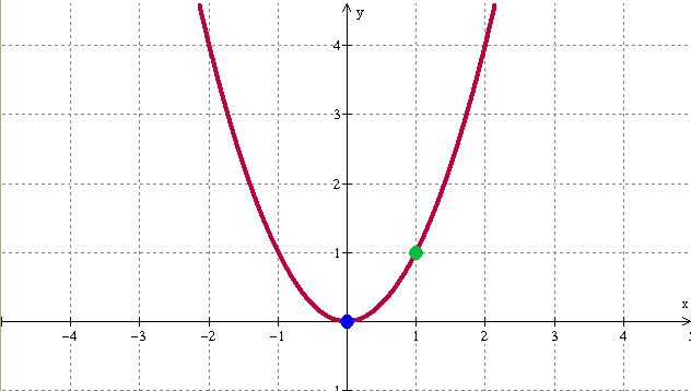
Let’s say we have the graph of y=x^2 and we want to find vectors normal to the curve at (0,0) and (1,1) (the blue and green dots).

parabola

Well, traditionally, we’d be crazy and parametrize the parabola by creating the vector-valued function \vec{r(t)}=<t,t^2> and then calculate the unit tangent vector (\vec{T}(t)=\frac{\vec{r}'(t)}{|\vec{r}'(t)|}) and then from that calculate the unit normal vector (\vec{N}(t)=\frac{\vec{T}'(t)}{|\vec{T}'(t)|}). [1] Then we’d calculate \vec{N}(0) and \vec{N}(1) to find the vectors.

But trust me, this is an awful amount of work, and \vec{N} is not a pretty function. We had to parametrize, take derivatives, and plug in values. And if you remember, we started out with such a simple equation y=x^2. Why can’t it be easier?

And it can. And this is where I need your help.

Instead of considering the plain old boring function y=x^2, we turn this into a surface by introducing a z direction: F(x,y)=y-x^2.

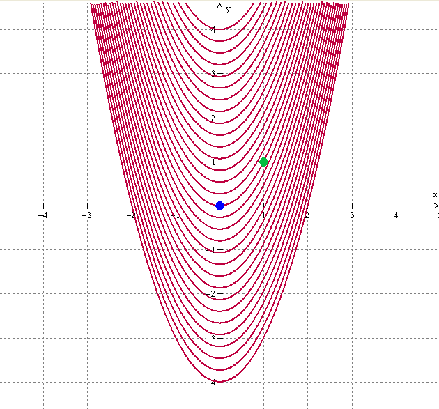
The function F(x,y) is a surface. We’re only interested in one slice of the surface, when F(x,y)=0 (when the height is 0). This will then reduce to our original equation y=x^2. The set of level curves of the surface is below. Note that the level curve that goes through the origin is the level curve we’re interested in.
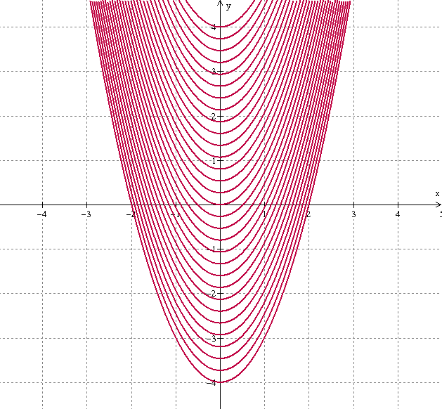
parabola-level-curves

Remember that one important (perhaps the most important) property of the gradient is that the gradient of a function points in the direction of maximum of steepness on a graph of level curves.

Let’s look at the points we’re interested in!

parabola-level-curves-dots

Just looking at the graph shows we’re onto something. Look at the blue dot. Which direction is the steepest, if you were standing at the blue dot and wanted to walk in the steepest direction? Well, clearly it would be directly north. (You want to walk the shortest distance to get to the next level curve. Since the change in heights between level curves is constant, you want to minimize the distance you’ve walked to get to the next height to have the steepest slope.) What about the green dot? Clearly, northwest.

And actually calculating the gradient of F(x,y) gives us \nabla F(x,y)=<-2x,1>.

At the blue dot, we get \nabla F(0,0)=<0,1>, which is a vector pointing straight up.

At the green dot, we get \nabla F(1,1)=<-2,1> which is a vector pointing northwest.

I’m plotting them below.

parabola-level-curves-dots-arrows

And without all the pesky level curves to distract us.

parabola-level-curves-dots-arrows-2

Clearly this method works. We take the original function y=x^2 and bring it into a higher dimension (F(x,y)=y-x^2). We use the fact that the gradient gives us the direction which is “steepest” on this surface, if we were trapped at a particular point. (In this case, (0,0) or (1,1). Notice these points lie on the level curve we care about, the level curve which actually is the equation we were initially concerned about (y=x^2). Then we recognize — somehow — that the gradient of the higher dimension equation somehow gives us the normal vector of the original equation we were concerned with.

The questions I have after doing this:

(1) Why did we have to change our nice curve y=x^2 into a surface F(x,y)=y-x^2 to solve this problem? And why this surface?

(2) How can we understand that the vector normal to the curve somehow is “magically” the gradient of the surface we created — one of whose level curves is the curve we’re interested in.

(3) Extending this analysis to problems where we want to find the normal vector to a surface like an ellipsoid (like 9x^2+4y^2+z^2=49) at a particular point, we’re going to be using the function F(x,y,z)=9x^2+4y^2+z^2-49 — whose level curves will be surfaces, stacked one on top of another. To find the normal vector, we take the point on the “level surface” which describes our ellispoid, and find the quickest way to get to the next “level surface”? Is that right? I think that seems right. Strange, but right.

(For a picture of some level surfaces, check it out here.)

Anyway, this is just my musings, my way of thinking through this. I’m not quite there. Any help you can give, great. If not, that’s cool too.

[1] I guess to make things simpler, we could simply calculate the direction of the normal vector and not worry about making it a unit normal vector, so we could simply calculate $\vec{T}'(t)$ only. We’re not concerned about the magnitude of the normal vector, only the fact that it’s normal.